In this document margin notes are used for code and comments that are not essential to the discussion, but that can still be interesting.
Gene expression
A gene expression experiment measures messenger RNA concentrations —or values correlated with RNA concentration, such as luminescence— for one or more genes under a specific condition. A series of experiments measure gene expression through several conditions.
Typically the results of a series of experiments is represented as a
matrix, with one row for each gene and one column for each condition. We
can find many experiments on NCBI Gene Expression Omnibus (GEO)
database. In this database each single experiment is called
sample and is identified with a code like
GSM2715492. All sample ids begin with prefix
GSM.
In the same way, series of experiments are called
series and are identified with codes starting
with GSE, such as GSE101789. We also find
platforms that describe the experimental
method: the microarray slide, the qPCR primers, or equivalent
characteristics. The platform can introduce some artifacts, so it is
important to only compare samples using the exact same platform.
Platforms ids begin with GPL, such as
GPL23823.
For this article we will use the series GSE101789 with
the gene expression of Pseudomonas syringae pv. tomato exposed
to light of different colors.
As you can guess, there are many ways to access NCBI GEO besides the
web interface. In R we can use the GEOquery libraryLibrary GEOquery is part of the
BioConductor toolkit. If needed, it should be installed
following the instructions on the website.
, but it is beyond the scope of this article. Each series
contains several components. We will care about three parts: the gene
expression in different experimental
conditions, the phenotypes — experimental
conditions—, and the features of each
gene.
To simplify this discussion I separated the components of the NCBI
GEO file in several plain text files. We start with the gene expression data, which
we load in R and we transform into a matrixThe commands read.delim() and
read.table() produce a data frame structure, which
works well with column data. We need to work with row
data, so it will be easier for us to use a matrix.
with the following code
ex <- read.delim("GSE101783_expression.txt")
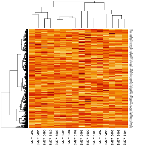
ex <- as.matrix(ex)The expression matrix has 15744 rows and 16 columns, so it is not practical to print it. Instead in Figure 1 we show a heat map of the matrix. Lighter colors represent higher gene expression. The dendrograms on the left side and above suggest how data can be clustered.
We can see that each column corresponds to a different sample. We would like to know the response of each gene to the experimental condition. Thus, we need to know the conditions of each experiment. In a gene expression experiment, the conditions or treatments can be for example:
- growth medium,
- environmental conditions, such as oxygen, light, temperature, or similar,
- time of exposure to the environment,
- healthy versus sick cells, as in the case of cancer,
- wild type cells versus mutant cells.
The file GSE101783_phenotype.txt
describes the experimental conditions for each sample in detail. We load
it with the following command, taking care of keeping text as
strings so we can handle the labels before creating the
factor variables.
phenotype <- read.delim("GSE101783_phenotype.txt", stringsAsFactors=FALSE)| geo_accession | treatment.ch1 |
|---|---|
| GSM2715489 | Darkness |
| GSM2715490 | Darkness |
| GSM2715491 | Darkness |
| GSM2715492 | Darkness |
| GSM2715493 | Blue light |
| GSM2715494 | Blue light |
| GSM2715495 | Blue light |
| GSM2715496 | Blue light |
| GSM2715497 | Red light |
| GSM2715498 | Red light |
| GSM2715499 | Red light |
| GSM2715500 | Red light |
| GSM2715501 | White light |
| GSM2715502 | White light |
| GSM2715503 | White light |
| GSM2715504 | White light |
The phenotype table has 16 rows —one for each experimental condition— and 39 columns, describing several characteristics. For this article we will care about one characteristic: treatment in channel 1, as shown in Table 1. More details can be seen at the end of this article, in the Appendix.
Our goal is to identify the underlying response of each gene to the
experimental condition. Thus, we prepare a factor to
describe the condition, taking the treatment.ch1
description and dropping the suffix " light".
Alternatively, we can create a factor manually, although it can be hard
to do it for large data sets.
condition <- factor(sub(phenotype$treatment.ch1,
                        pattern = " light", replacement = ""))
For the rest of this article we will focus on two arbitrary genes,
chosen only as good examples. They correspond to expression matrix’s
rows 1159 and 3342. To give a name to these genes we need to load the
file GPL23823_features.txt
with the gene descriptions. As before, there are several columns, but we
will only show the gene description.
features <- read.delim("GPL23823_features.txt")
features[c(1159, 3342), c("ORF", "DESCRIPTION")]| ORF | DESCRIPTION | |
|---|---|---|
| 1159 | PSPTO_2413 | PSPTO_2413;Product: urease accessory protein UreE |
| 3342 | PSPTO_5142 | PSPTO_5142;Product: hypothetical protein |
We will model the gene expression as the sum of two components: an underlying condition-dependent expression level, and a noise component independent of the experimental condition. We want to identify the first component and control the second one. Moreover, we want to see if the underlying expression level changes when conditions change.
Expression analysis of gene 1159 (PSPTO_2413)
Table 2 and Figure 2 show the expression level of gene 1159 (PSPTO_2413) and the corresponding condition on each sample.
| expression | condition | |
|---|---|---|
| GSM2715489 | 8.65 | Darkness |
| GSM2715490 | 8.66 | Darkness |
| GSM2715491 | 9.12 | Darkness |
| GSM2715492 | 9.19 | Darkness |
| GSM2715493 | 9.48 | Blue |
| GSM2715494 | 8.48 | Blue |
| GSM2715495 | 9.14 | Blue |
| GSM2715496 | 8.35 | Blue |
| GSM2715497 | 7.58 | Red |
| GSM2715498 | 11.27 | Red |
| GSM2715499 | 8.39 | Red |
| GSM2715500 | 8.27 | Red |
| GSM2715501 | 8.77 | White |
| GSM2715502 | 9.02 | White |
| GSM2715503 | 9.16 | White |
| GSM2715504 | 8.76 | White |

Linear model without intercept
We want to know what is the expression of gene 1159 under each condition and compare them. As discussed in a previous article, we can find the gene expression for each condition with a linear model without intercept.
model0 <- lm(ex[1159,] ~ condition + 0)
summary(model0)| Estimate | Std. Error | t value | Pr(>|t|) | ||
|---|---|---|---|---|---|
| conditionBlue | 8.863 | 0.439 | 20.19 | 1.25e-10 | * * * |
| conditionDarkness | 8.905 | 0.439 | 20.29 | 1.182e-10 | * * * |
| conditionRed | 8.878 | 0.439 | 20.22 | 1.225e-10 | * * * |
| conditionWhite | 8.928 | 0.439 | 20.34 | 1.147e-10 | * * * |
The fitted model’s coefficients correspond to the mean expression
level for each condition. Each 𝑝-value corresponds to the null
hypothesis “real gene expression is zero”You can find several web pages with
refreshers about 𝑝-values and statistical significance on the
web.
. As expected, all 𝑝-values are small, since the gene is
expressed in all conditions.
The stars in the last columns are used to show which 𝑝-values are below the traditional thresholds. Three stars means 𝑝-value below 1%, two stars represent “under 5%”, and so on.
One way to understand the model is the following diagram. Each arrow represents one comparison made when we fit the linear model.

In this basic case, each circle represent the average expression for each condition, and the arrows represent the estimation calculated by fitting the linear model. It is important to know that we can have only four arrows in this diagram, since we have four conditions, and that limits how many combinations we can take.
The expression levels are hard to interpret without context. Are they high or low? The mean values are different. Are they significantly different? In other words, are the underlying expression levels really different, or the difference of means corresponds only to the noise?
Linear model with intercept
To answer these questions it is more useful to fit a linear model with intercept, that will show the difference between a reference condition against all other conditions.
model1 <- lm(ex[1159,] ~ condition)
summary(model1)| Estimate | Std. Error | t value | Pr(>|t|) | ||
|---|---|---|---|---|---|
| (Intercept) | 8.863 | 0.439 | 20.19 | 1.25e-10 | * * * |
| conditionDarkness | 0.0425 | 0.6208 | 0.06846 | 0.9465 | |
| conditionRed | 0.015 | 0.6208 | 0.02416 | 0.9811 | |
| conditionWhite | 0.065 | 0.6208 | 0.1047 | 0.9183 |
The intercept shows the expression level of the reference condition. Again, we can represent this model with a diagram.

In this case the reference is automatically chosen to be “the first
level of the condition factor”, which in this case is
Blue. This is because, unless we say otherwise, the factor
levels are sorted alphabetically.
levels(condition)[1] "Blue" "Darkness" "Red" "White" This does not necessarily corresponds to the most interesting
questionThis is the key question.
. We need a way to choose the reference
level.
Choosing the reference level
There are several ways to choose the reference level. We will discuss
some of the easy methods. The easiest one is to use the function
relevel() to create a new factor with the same levels in
different order.
From the the sake of argument I will assume that a good reference
level is "Darkness". Thus, the new factor will be called
dark_vs_. We create and examine it as follows.
dark_vs_ <- relevel(condition, "Darkness")
levels(dark_vs_)
[1] "Darkness" "Blue" "Red" "White" We see that this new factor dark_vs_ contains the same
values as the old factor condition, but the levels are in a
different order. Now we can fit the linear model again.
model2<- lm( ex[1159,] ~ dark_vs_ )summary(model2)| Estimate | Std. Error | t value | Pr(>|t|) | ||
|---|---|---|---|---|---|
| (Intercept) | 8.905 | 0.439 | 20.29 | 1.182e-10 | * * * |
| dark_vs_Blue | -0.0425 | 0.6208 | -0.06846 | 0.9465 | |
| dark_vs_Red | -0.0275 | 0.6208 | -0.0443 | 0.9654 | |
| dark_vs_White | 0.0225 | 0.6208 | 0.03624 | 0.9717 |
In the new results the intercept shows the expression level
for "Darkness", and the other coefficients show the
differential expression for "Blue", "Red" and
"White" light.

Why doing this complicated way? We could just calculate the difference between the averages? Because of the 𝑝-values. This time the null hypothesis is “the expression levels are the same”. Small 𝑝-values show that we do not have enough evidence to reject the null hypothesis. In other words, there is no statistically significant difference between the expression levels. The gene 1159 does not respond to the light.
Expression analysis for gene 3342 (PSPTO_5142)
For comparison, let us see the case of gene 3342, which has the following expression levels.

Using the same modified factor dark_vs_, this time we
get these results
model3 <- lm(ex[3342,] ~ dark_vs_)
summary(model3)| Estimate | Std. Error | t value | Pr(>|t|) | ||
|---|---|---|---|---|---|
| (Intercept) | 13.74 | 0.146 | 94.14 | 1.38e-18 | * * * |
| dark_vs_Blue | -2.875 | 0.2065 | -13.92 | 9.078e-09 | * * * |
| dark_vs_Red | -2.877 | 0.2065 | -13.94 | 8.989e-09 | * * * |
| dark_vs_White | 0.7775 | 0.2065 | 3.765 | 0.002694 | * * |
This time all the differences are statistically significant. Moreover, we know that gene 3342 is repressed under blue or red light, and it is activated under white light. It is easy to find confidence intervals for the change in expression.
confint(model3, level=0.99)| 0.5 % | 99.5 % | |
|---|---|---|
| (Intercept) | 13.2990193 | 14.190981 |
| dark_vs_Blue | -3.5057119 | -2.244288 |
| dark_vs_Red | -3.5082119 | -2.246788 |
| dark_vs_White | 0.1467881 | 1.408212 |
Using Contrast matrices
There is another approach to compare gene expressions, more flexible than just reorganizing factor levels. As usual, higher flexibility implies higher complexity.
To make the example more clear, we use the original
condition factor, without reordering.
The function contr.treatment() can be used to create a
contrasts matrix, like this.
contrast1 <- contr.treatment(levels(condition), base = 2)contrast1| Blue | Red | White | |
|---|---|---|---|
| Blue | 1 | 0 | 0 |
| Darkness | 0 | 0 | 0 |
| Red | 0 | 1 | 0 |
| White | 0 | 0 | 1 |
This function takes the names of factor’s levels and the number
indicating the base level used for reference. The resulting
contrasts matrix has one row and one column for each level of
condition, except that there is no column for the base
level. The row that only has zeros will be the base level.
Now when we fit the linear model we need to include a
contrasts= option. This option takes a list, where
each element has the name of a factor. There can be several factors in a
model, each one with its own contrast. In our case we have only one
factor.
model3b <- lm(ex[3342,] ~ condition, contrasts = list(condition=contrast1))summary(model3b)| Estimate | Std. Error | t value | Pr(>|t|) | ||
|---|---|---|---|---|---|
| (Intercept) | 13.74 | 0.146 | 94.14 | 1.38e-18 | * * * |
| conditionBlue | -2.875 | 0.2065 | -13.92 | 9.078e-09 | * * * |
| conditionRed | -2.877 | 0.2065 | -13.94 | 8.989e-09 | * * * |
| conditionWhite | 0.7775 | 0.2065 | 3.765 | 0.002694 | * * |
We see that we recovered the same result as model3
without re-leveling the factor. It is more complicated, but will have
some advantages.
Making the contrast matrix manually
Once we know how the contrast matrix looks, we can make it manually.
In R we use matrix(data, nrow, byrow) to create a new
matrix from a vector data. If we do not include
byrow=TRUE then the matrix will be filled by columns. Try
it and see the difference.
The code to make a matrix like contrast1 is this
contrast2 <- matrix(
c(1,0,0,
  0,0,0,
  0,1,0,
  0,0,1), nrow=4, byrow=TRUE)
colnames(contrast2) <- c("B_D","R_D","W_D")
rownames(contrast2) <- levels(condition)contrast2| B_D | R_D | W_D | |
|---|---|---|---|
| Blue | 1 | 0 | 0 |
| Darkness | 0 | 0 | 0 |
| Red | 0 | 1 | 0 |
| White | 0 | 0 | 1 |
Obviously, it produces the same model and the same coefficients as before.
Other combinations
We can make other contrast matrices, but there are technical constraints on what can be done. One way to easy avoid these contrast is to build a single comparison. For example, an important biological issue is to compare the gene expression under blue light versus under red light, and find if the difference is statistically significant.
To answer this question we build a one-column matrix with a code like this
contrast3 <- matrix(c( 1/2, 0,-1/2, 0), nrow=4)
colnames(contrast3) <- c("B-R")
rownames(contrast3) <- levels(condition)
which produces the following matrix
contrast3| B-R | |
|---|---|
| Blue | 0.5 |
| Darkness | 0.0 |
| Red | -0.5 |
| White | 0.0 |
Not the fitted model has only two coefficients
model5 <- lm(ex[3342,] ~ condition,
 contrasts=list(condition=contrast3))
summary(model5)| Estimate | Std. Error | t value | Pr(>|t|) | ||
|---|---|---|---|---|---|
| (Intercept) | 12.5 | 0.4476 | 27.93 | 1.117e-13 | * * * |
| conditionB-R | 0.0025 | 1.266 | 0.001975 | 0.9985 |
Now it will be useful to keep in mind the mean expression for each condition.
tapply(ex[3342,], condition, mean) Blue Darkness Red White
10.8700 13.7450 10.8675 14.5225 Close inspection shows that coefficient conditionB-R is
the difference between mean expression in "Blue" and
"Red" conditions. More importantly, we get a 𝑝-value for
the difference. We conclude that, although "Blue" and
"Red" are different from "Darkness".
We also observe that the intercept is the mean of all expressions.
mean(ex[3342,])[1] 12.50125Unfortunately it is not easy to do this comparison for several conditions at the same time. For this article we will limit us to only one comparison per linear model.
All versus the average
We have the mean expression for each condition and the global mean of all expressions. It is easy to calculate the difference between the global mean and the mean of each condition.
tapply(ex[3342,], condition, mean) - mean(ex[3342,]) Blue Darkness Red White
-1.63125 1.24375 -1.63375 2.02125 It is not so easy to see if this difference is significant. We can
answer this question using contrast matrices created with the
contr.sum() function.
contrast4 <- contr.sum(levels(condition))
colnames(contrast4) <- c("B","D","R")
The contr.sum() does not assign names to the columns, so
we assign them manually. The resulting matrix is this
contrast4| B | D | R | |
|---|---|---|---|
| Blue | 1 | 0 | 0 |
| Darkness | 0 | 1 | 0 |
| Red | 0 | 0 | 1 |
| White | -1 | -1 | -1 |
We see that the last row is different from the rest, and indeed it is not included in the output. This is always the case when we do not have enough degrees of freedom. Since we are comparing to the average, we lose one degree of freedom. We can represent this model with the following diagram.

As before, we can have up to four arrows —that is, contrasts— given that we are limited by the number of conditions. To include the mean we must “sacrifice” one of the conditions to make space for the average. The “lost” row is replaced with a row of -1.
The fitted model has the following coefficients
model6 <- lm(ex[3342,] ~ condition,
 contrasts=list(condition=contrast4))
summary(model6)| Estimate | Std. Error | t value | Pr(>|t|) | ||
|---|---|---|---|---|---|
| (Intercept) | 12.5 | 0.073 | 171.2 | 1.057e-21 | * * * |
| conditionB | -1.631 | 0.1264 | -12.9 | 2.15e-08 | * * * |
| conditionD | 1.244 | 0.1264 | 9.836 | 4.279e-07 | * * * |
| conditionR | -1.634 | 0.1264 | -12.92 | 2.113e-08 | * * * |
We observe that the intercept is the global average, and the rest of the coefficients are the difference between the average and the average expression under each condition. Also, we have 𝑝-values to evaluate the statistical significance of each difference.
How would you make a contrast matrix to compare the global average to “Blue”, “Red” and “White”, omitting “Darkness”?
Appendix: Materials & Methods
Just to make my biologist friend happy, we can see more details about the experimental protocol as described in the first row of phenotype file.
phenotype[1, 3:31]| status | submission_date | last_update_date | type |
|---|---|---|---|
| Public on Oct 01 2018 | Jul 23 2017 | Oct 01 2018 | RNA |
| channel_count | source_name_ch1 | organism_ch1 |
|---|---|---|
| 1 | Wild type 10 min Dark | Pseudomonas syringae pv. tomato str. DC3000 |
| characteristics_ch1 | characteristics_ch1.1 | characteristics_ch1.2 |
|---|---|---|
| genotype/variation: Wild type | culture type: Liquid | treatment: Darkness |
| characteristics_ch1.3 | growth_protocol_ch1 | molecule_ch1 |
|---|---|---|
| treatment duration: 10 min | Transcriptomic analyses were done with cultures grown in liquid KB medium. Total RNA was extracted from cell cultures collected at O.D.=0.5 after a 10 min treatment with either white, blue or red light. Cultures maintained in the darkness were used as controls. | total RNA |
| extract_protocol_ch1 | label_ch1 | label_protocol_ch1 |
|---|---|---|
| Total RNA from four biological replicates from each treatment was extracted with TRI Reagent (Ambion) as recommended by the manufacturer. RNA was pre-treated with RNase-free DNase I (Roche) plus RNaseOUT (Invitrogen), followed by purification with RNeasy columns (Qiagen). | Cy3 | cDNA was labeled with Cy3 by using the SuperScript III indirect cDNA labeling system (Invitrogen) as described in the instruction manual (One-Color Microarray Based Gene Expression Analysis Manual). |
| taxid_ch1 | hyb_protocol | scan_protocol |
|---|---|---|
| 223283 | 600 ng of Cy3 probes were mixed and added to 5 μl of 10x Blocking Agent and Nuclease-free water in a 25 μl reaction. Then, we added 25 μl from 2x GExHybridization buffer and mixed carefully. The samples were placed on ice and quickly loaded onto arrays, hybridized at 65 ºC for 17 h and then washed once in GE wash buffer 1 at room temperature (1 min) and once in GE Wash Buffer 2 at 37 ºC (1 min). | Images from Cy3 channel were equilibrated and captured with a High resolution Scanner (Agilent) and spots quantified using Feature Extraction software (Agilent). |
| description | description.1 | data_processing |
|---|---|---|
| G0 | Gene expression after 10 min darkness treatment. | For local background correction and normalization, the methods normexp and loess in LIMMA were used, respectively. Log-ratio values were scaled using as scale estimator the median-absolute-value. Linear model methods were used for determining differentially expressed genes. Each probe was tested for changes in expression over replicates by using an empirical Bayes moderated t-statistic. To control the false discovery rate, p-values were corrected by using the method of Benjamani and Hochberg, 1995. The expected false discovery rate (FDR) was controlled to be less than 1%. |
| platform_id | contact_name | contact_email |
|---|---|---|
| GPL23823 | Emilia,,López Solanilla | emilia.lopez@upm.es |
| contact_institute | contact_address |
|---|---|
| CBGP-Universidad Politécnica de Madrid (UPM) | Parque Científico y Tecnológico UPM, Campus de Montegancedo, Ctra. M-40, km 38 |
| contact_city | contact_state |
|---|---|
| Pozuelo de Alarcon | Madrid |