What happens when 𝑛 is big?
A simple model
Now we have a coin 𝑋 with two possible outcomes: +1 and -1
To make life easy, we assume 𝑝=0.5
What are the expected value and variance of X ?
Throw the coin 𝑛 times
We throw the coin 𝑛 times, and we calculate 𝑌, the sum of all 𝑋 \[Y=\sum_{i=1}^𝑛 X_i\]
What are the expected value and variance of 𝑌 ?
It is easy to see that
- \(𝑌\) is basically a Binomial
random variable
- \(𝔼 𝑌 = 0,\) because \(𝔼 𝑋 = 0\)
- \(𝕍 𝑌 = 𝑁,\) because \(𝕍 𝑋 = 1\)
Fix the variance to 1
Now consider \(Z_n=Y/\sqrt{𝑛}\)
It is easy to see that \(𝔼Z_n = 0\)
and \(𝕍Z_n = 1\) independent of 𝑛
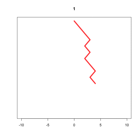
The possible values of \(Z_n\) are
not integers. Not even rationals
What happens with \(Z_n\) when 𝑛 is
really big?
Variance 1, M=5
![]()
Variance 1, M=50
![]()
Variance 1, M=500
![]()
Variance 1, M=5000
![]()
When M is big, we get a Normal distribution
![]()
The Normal distribution
This “bell-shaped” curve is found in many experiments, especially
when they involve the sum of many small contributions
- Measurement errors
- Height of a population
- Scores on University Admission exams
It is called Gaussian distribution, or also Normal
distribution
Normal distribution
![]()
Here outcomes are real numbers
Any real number is possible
Probability of any \(x\) is zero
(!)
We look for probabilities of intervals
The Central Limit Theorem
“The sum of several independent random variables
converges to a Normal distribution”
The sum should have many terms, they should be independent, and they
should have a well defined variance
(In Biology sometimes the variables are not independent, so be
careful)
Central limit theorem
When \(n→∞,\) the distribution of
\(Z_n=∑ X/\sqrt{𝑛}\) will converge to a
Normal distribution \[\lim_{n→∞} Z_n ∼ Normal(0,1)\]
More in general
If \(X_i\) is a set of i.i.d. random
variables, with \[𝔼X_i=μ\quad\text{and}\quad
𝕍X_i=σ^2\quad\text{for all }i\] then, when \(n\) is large \[\lim_{n→∞} \frac{\sum_i X_i-μ}{σ\sqrt{𝑛}} ∼
\text{Normal}(0,1)\]
In other words
If \(X_i\) is a set of i.i.d. random
variables, with \[𝔼X_i=μ\quad\text{and}\quad
𝕍X_i=σ^2\quad\text{for all }i\] then, when \(n\) is large \[\lim_{n→∞} \frac{\sum_i X_i-μ}{\sqrt{𝑛}} ∼
\text{Normal}(0, σ^2)\]
This is why Normal distributions are
important
Noise is usually Normal
- Thermal noise is the sum of many small vibrations in all directions
- they sum and usually cancel each other
- Phenotype depends on several genetic conditions
- Height, weight and similar attributes depend on the combination of
several attributes
It does not always work
- Not all combined effects are sums
- some effects are multiplicative
- Some effects may not have finite variance
- sometimes variance is infinite
- Not all effects are independent
- this is the most critical issue
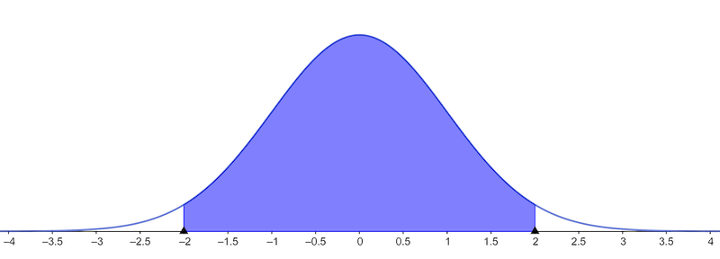
Probabilities of Normal Distribution
![]()
≈95% of normal population is between \(-2\cdot\text{sd}(\mathbf x)\) and \(2\cdot\text{sd}(\mathbf x)\)
≈99% of normal population is between \(-3\cdot\text{sd}(\mathbf x)\) and \(3\cdot\text{sd}(\mathbf x)\)