What is a measurement?

• A measurement tells us about a property of something

  • It gives a number to that property

• Measurements are always made using an instrument

  • Rulers, stopwatches, scales, thermometers, etc.

• The result of a measurement has two parts:

  • A number and a unit of measurement

What is not a measurement?

There are some processes that might seem to be measurements, but are not. For example

• Counting is not normally viewed as a measurement
• Tests that lead to a ‘yes/no’ answer or a ‘pass/fail’ result
• Comparing two pieces of string to see which one is longer

However, measurements may be part of the process of a test

Uncertainty must be declared

How big is the margin? How bad is the doubt?

We declare an interval: \([x_\text{min}, x_\text{max}]\)

Most of the time we write x ± 𝚫x

Example: 20cm ± 1cm

Error versus uncertainty

Do not to confuse error and uncertainty

Error is the difference between the measured and the “true” value

Uncertainty is a quantification of the doubt about the result

Whenever possible we try to correct for any known errors

But any error whose value we do not know is a source of uncertainty

Flaws in the measurement can come from

• The measuring instrument

• The item being measured

• The measurement process

• ‘Imported’ uncertainties

• Operator skill

• Sampling issues

• The environment

The measuring instrument

instruments can suffer from errors including

• wear,

• drift,

• poor readability,

• noise,

• etc.

The item being measured

The thing we measure may not be stable

For example, when we measure the size of an ice cube in a warm room

The measurement process

The measurement itself may be difficult to make

Measuring the weight of small animals presents particular difficulties

‘Imported’ uncertainties

Calibration of your instrument has an uncertainty

Operator skill

One person may be better than another at reading fine detail by eye

The use of an a stopwatch depends on the reaction time of the operator

Sampling issues

The measurements you make must be representative

If you are choosing samples from a production line, don’t always take the first ten made on a Monday morning

The environment

• Temperature

• Air pressure

• Humidity

and many other conditions can affect the measuring instrument or the item being measured

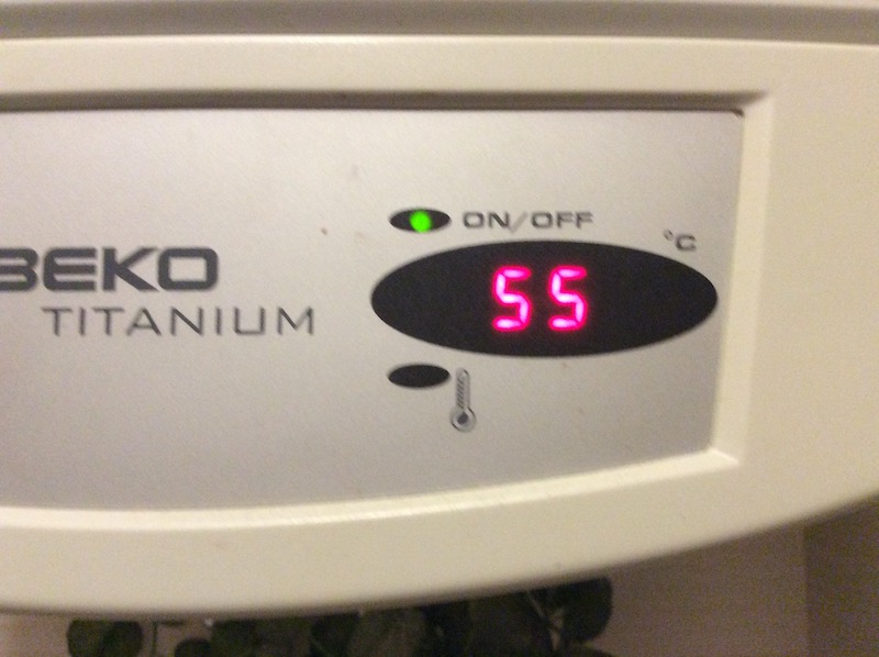
Real vs measured value

If it shows 55°C, the real temperature is somewhere between 53°C and 57°C

We write 55°C ± 2.5°C

For a single read, 𝚫x = half of the resolution

This is a “one time” error

• We notice it immediately
• It does not change if we measure again

Two kinds of observational error

Every time we repeat a measurement with a sensitive instrument, we obtain slightly different results

• Systematic error which always occurs, with the same value, when we use the instrument in the same way and in the same case

• Random error which may vary from observation to another

Two ways to estimate uncertainties

• Type A - uncertainty estimates using statistics

  • (usually from repeated readings)

• Type B - uncertainty estimates from any other information.

  • past experience of the measurements, calibration certificates, manufacturer’s specifications, calculations, published information, common sense

In most measurement situations, uncertainty evaluations of both types are needed

Combining Uncertainty

Sum of two measurements:
\[(x ± 𝚫x) + (y ± 𝚫y) = (x+y) ± (𝚫x+𝚫y)\]

Difference between measurements:
\[(x ± 𝚫x) - (y ± 𝚫y) = (x-y) ± (𝚫x+𝚫y)\]

Multiplying Uncertainty

To calculate \((x ± 𝚫x) × (y ± 𝚫y)\) we first write the uncertainty as percentage

\[(x ± 𝚫x/x\%) × (y ± 𝚫y/y\%)\]

Then we sum the percentages:
\[xy ± (𝚫x/x + 𝚫y/y)\%\]

Finally we convert back to the original units:
\[xy ± xy(𝚫x/x + 𝚫y/y)\]

General formula

Assuming that the errors are small compared to the main value, we can find the error for any “reasonable” function

Taylor’s Theorem says that, for any derivable function \(f,\) we have

\[ f(x±𝚫x) = f(x) ± \frac{df}{dx}(x)\cdot 𝚫x + \frac{d^2f}{dx^2}(x+\varepsilon)\cdot \frac{𝚫x^2}{2} \]

When \(𝚫x\) is small, we can ignore the last part.

Example 1

\[ \begin{aligned} (x ±𝚫x)^2& ≈ x^2 ± 2x\cdot𝚫x\\ & = x^2 ± 2x^2\cdot\frac{𝚫x}{x} \\ & = x^2 ± 2𝚫x\% \end{aligned} \]

because \[\frac{dx^2}{dx}=2x\]

Example 2

\[ \begin{align} \sqrt{x ±𝚫x}& ≈ \sqrt x ± \frac{1}{2\sqrt x}\cdot 𝚫x\\ & = \sqrt x ± \frac{1}{2}\sqrt x\cdot \frac{𝚫x}{x}\\ & = \sqrt x ± \frac{1}{2}𝚫x\% \end{align} \]

because \[\frac{d\sqrt x}{dx}=\frac 1 {2\sqrt x}\]

Variance quantifies uncertainty

In this case, the value \(Δx\) will represent the standard deviation of the measurement

The standard deviation is the square root of the variance

Then, we combine variances using the rule

“The variance of a sum is the sum of the variances”

(Again, this is valid only if the errors are independent)

The probabilistic rule

\[ \begin{align} (x ± Δx) + (y ± Δy) & = (x+y) ± \sqrt{Δx^2+Δy^2}\\ (x ± Δx) - (y ± Δy) & = (x-y) ± \sqrt{Δx^2+Δy^2}\\ (x ± Δx\%) \times (y ± Δy\%)& =x y ± \sqrt{Δx\%^2+Δy\%^2}\\ \frac{x ± Δx\%}{y ± Δy\%} & =\frac{x}{y} ± \sqrt{Δx\%^2+Δy\%^2} \end{align} \]

Confidence interval for the measurement

When using probabilistic rules we need to multiply the standard deviation by a constant k, associated with the confidence level

In most cases (but not all), the uncertainty follows a Normal distribution. In that case

• \(k=1.96\) corresponds to 95% confidence
• \(k=2.00\) corresponds to 98.9% confidence
• \(k=2.57\) corresponds to 99% confidence
• \(k=3.00\) corresponds to 99.9% confidence