Class 3: Interval Arithmetic
Methodology of Scientific Research
Andrés Aravena, PhD
February 27, 2024
Math in a napkin
(or in the back of an envelope)
Estimating order of magnitude
At first, we go by powers of ten \[10^{-1}, 10^{0}, 10^{1}, 10^{2}, 10^{3}\] This is very “low resolution”
To do better, we can increment the exponent by 0.5 \[10^{-1}, 10^{-0.5}, 10^{0}, 10^{0.5}, 10^{1}\]
Since \(10^{0.5} = \sqrt{10}≈ 3.16≈3\) we can say \[0.1, 0.3, 1, 3, 10, 30, 100,…\]
Fine tuning estimations
To have higher resolution, we can combine two guesses
- \(A\): A power of ten that is maybe too small
- \(B\): A power of ten that is maybe too big
Since we are using powers, the “average” is the geometric mean \[C=\sqrt{A⋅B}\] because \[\log C=\frac{\log A + \log B}2\]
Easy approximation of geometric mean
This can be approximated taking the average of the mantisas and the average of the exponents
If \(A=a× 10^x\) and \(B=b×10^y\) then \[\begin{aligned} \sqrt{A⋅B}&=\sqrt{a⋅b×10^{x+y}}\\ &=\sqrt{a⋅b}×10^{\frac{x+y}2}\\ &\approx \frac{a+b}{2}×10^{\frac{x+y}2} \end{aligned} \] when \(a\) and \(b\) are between 1 and 9
Practice
What is the weight of this ferry?
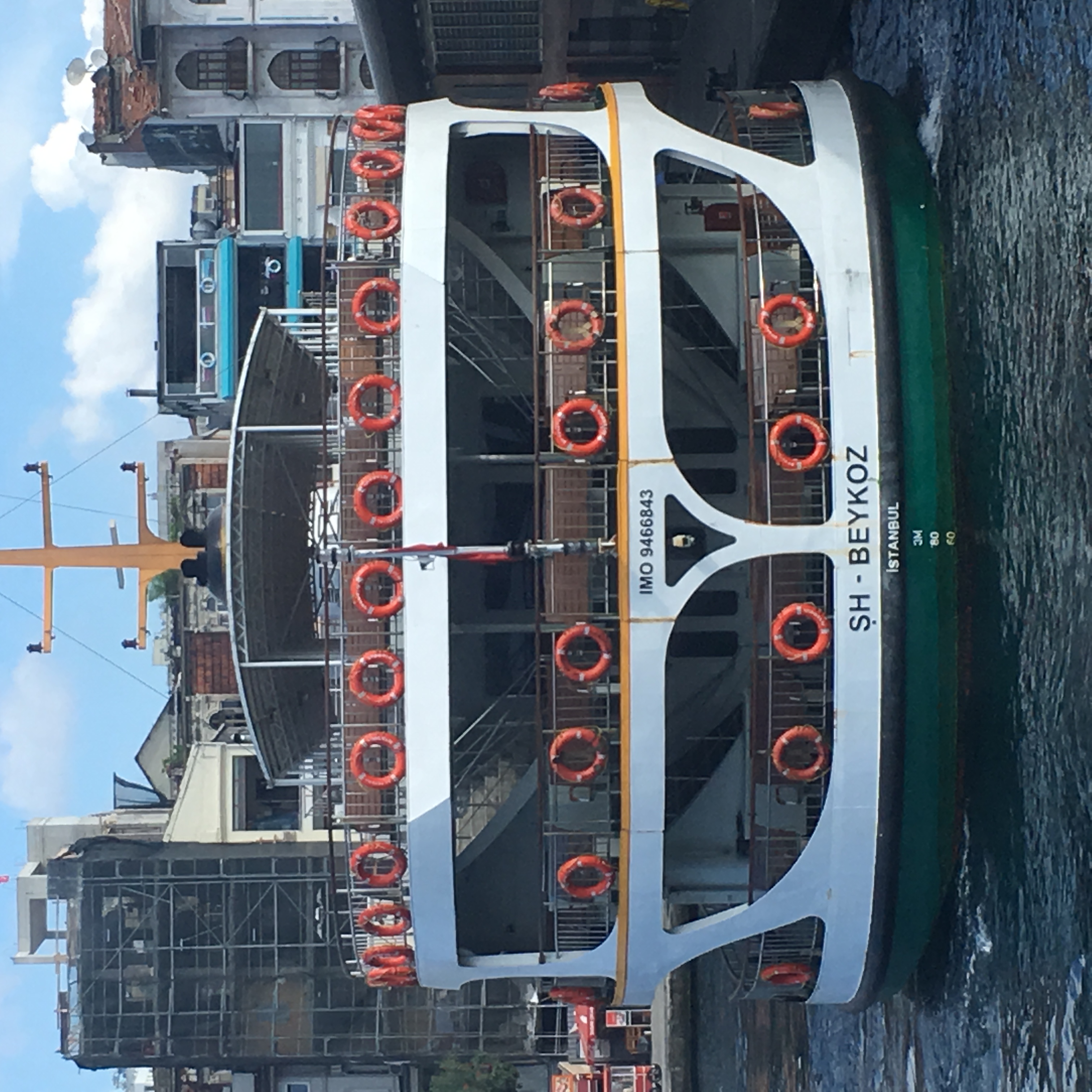
Side view

Another side view

More Practice
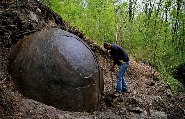
Massive Stone Ball Discovered by Bosnian
In 2016 a large stone ball was found in Podubravlje village near Zavidovici, Bosnia and Herzegovina.
Souvenirs for Tourists
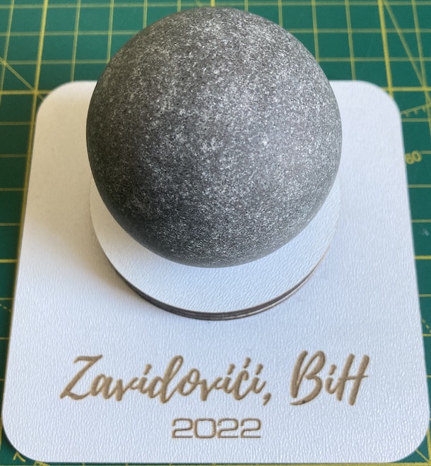
We do not know how these stones were made
Similar stones have been found in Costa Rica
Nevertheless, people have made small round stones to sell as souvenirs
Density of the stone ball
I was given a stone ball from Bosnia
We want to know its density
So we need to know mass and volume
- Estimate its mass
- Estimate its volume
- Estimate its density
Ask questions
Our estimation of mass
Based on intuition we think that the mass is more than 100gr and less than 1Kg
Taking the geometric mean, we got 300gr
But it can be anything between 200gr and 400gr
We write 300gr ± 100gr
Our estimation of volume
Comparing with a tea cup, we guess 80ml
But it can be anything between 70ml and 90ml
We write 80ml ± 10ml
How would you estimate the density?
How can we improve our margin of error?
Interval arithmetic
Definitions
We will represent measurements as intervals \([x_1, x_2]\)
A binary operation \(\star\) on two intervals is defined by
\[[x_1, x_2] {\,\star\,} [y_1, y_2] = \{ x \star y \, | \, x \in [x_1, x_2] \text{ and } y \in [y_1, y_2] \}.\]
In other words, it is the set of all possible values of \(x \star y\),
where \(x\) and \(y\) are in their corresponding
intervals.
Wikipedia: “Interval arithmetic”
Simplification for basic operations
If \(\star\) is either \(+, -, \cdot,\) or \(÷\), then \([x_1, x_2] \star [y_1, y_2]\) is \[ [\min\{ x_1 \star y_1, x_1 \star y_2, x_2 \star y_1, x_2 \star y_2\},\\ \max \{x_1 \star y_1, x_1 \star y_2, x_2 \star y_1, x_2 \star y_2\} ], \] as long as \(x \star y\) is defined for all \(x\in [x_1, x_2]\) and \(y \in [y_1, y_2]\).
Even easier
- Addition: \[[x_1, x_2] + [y_1, y_2] = [x_1+y_1, x_2+y_2]\]
- Subtraction: \[[x_1, x_2] - [y_1, y_2] = [x_1-y_2, x_2-y_1]\]
Multiplication
This is the area of a rectangle with varying edges
\([x_1, x_2] \cdot [y_1, y_2]\) is \[[\min \{x_1 y_1,x_1 y_2,x_2 y_1,x_2 y_2\},\\ \max\{x_1 y_1,x_1 y_2,x_2 y_1,x_2 y_2\}]\]
The result interval covers all possible areas, from smallest to the largest
Division needs more attention
\[\frac{[x_1, x_2]}{[y_1, y_2]} = [x_1, x_2] \cdot \frac{1}{[y_1, y_2]},\] where \[\begin{aligned} \frac{1}{[y_1, y_2]} &= \left[\tfrac{1}{y_2}, \tfrac{1}{y_1} \right] \textrm{ if }\;0 \notin [y_1, y_2]\\ \frac{1}{[y_1, 0]} &= \left[-\infty, \tfrac{1}{y_1} \right] \end{aligned}\]
finally
\[\begin{aligned} \frac{1}{[0, y_2]} &= \left [\tfrac{1}{y_2}, \infty \right ] \\ \frac{1}{[y_1, y_2]} &= \left [-\infty, \tfrac{1}{y_1} \right ] \cup \left [\tfrac{1}{y_2}, \infty \right ] \textrm{ if }\;0 \in (y_1, y_2) \end{aligned}\]
Functions
- Exponential function: \(a^{[x_1, x_2]} = [a^{x_1},a^{x_2}]\) for \(a > 1,\)
- Logarithm: \(\log_a [x_1, x_2] = [\log_a {x_1}, \log_a {x_2}]\) for positive intervals \([x_1, x_2]\) and \(a>1,\)
- Odd powers: \([x_1, x_2]^n = [x_1^n,x_2^n]\), for odd \(n\in ℕ\)
What happens in even powers?
Density of the stone ball
Measuring the diameter
Let’s measure the diameter using a caliper
It is about 5.3cm
Since the ball is not 100% spherical, the diameter varies between 5.2cm and 5.4cm
Now we can calculate the volume using the formula \[\frac{4}{3} π r^3\]
Calculating the volume
Using the central value
[1] 2.65[1] 77.95181Being pessimistic
Maybe the diameter is 5.2cm. Then
[1] 73.62218Being optimistic
Maybe the diameter is 5.4cm. Then
[1] 82.44796A range of possibilities
The real volume is somewhere in the range
[1] 73.62218 82.44796That is, an interval with center
[1] 78.03507and width
[1] 4.41289Two possible centers
Notice that
[1] 78.03507is not the same as
[1] 77.95181but both values are close (why?)
For now we take the first one
How many decimals?
We can write 78.0350671 ± 4.4128905 cm3
But then, most of the decimals are meaningless
We get a false feeling of precision,
but we really do not know all the decimals
Rounding numbers
First, we round the error term to a single digit
[1] 4Then we discard all decimals smaller than the error term
[1] 78so we write 78 ± 4cm3
(we get the same result if we use vol)
Evaluating the density
Each measurement is an interval
We have \[\text{vol}=78\text{cm}^3 ± 4\text{cm}^3\] and \[\text{mass}=250\text{gr} ± 50\text{gr}\]
Now we can calculate the density
We will consider all possible cases
Intervals
\[\begin{aligned} \text{vol} &=[74, 82]\text{cm}^3\\ \text{mass}&=[200, 300]\text{gr}\\ \text{density}_{\min} &=\min \left\{\frac{200}{74}, \frac{300}{74},\frac{200}{82},\frac{300}{82}\right\}\frac{\text{gr}}{\text{cm}^3}\\ \text{density}_{\max} &=\max\left\{\frac{200}{74}, \frac{300}{74},\frac{200}{82},\frac{300}{82}\right\}\frac{\text{gr}}{\text{cm}^3}\ \end{aligned} \]
Calculating
\[\text{density}=[2.4390244, 4.0540541] \frac{\text{gr}}{\text{cm}^3}\] Rounding, we get \[\text{density}=[2.4, 4.1] \frac{\text{gr}}{\text{cm}^3}\]
Summary
- Train your instinct
- If you can, think slow
- Every measurement is an interval
- All calculations yield an interval
- Find the margin of error
- Omit decimals smaller than the margin of error
- Intervals can be written \([x_{min}, x_{max}]\) or \(x_{mean}±\Delta x\)
Apply to Drake equation
\[N = R_* \cdot f_\mathrm{p} \cdot n_\mathrm{e} \cdot f_\mathrm{l} \cdot f_\mathrm{i} \cdot f_\mathrm{c} \cdot L\]
- \(R_{*}\) = 1 yr-1
- \(f_{p}\) = 0.2 to 0.5
- \(n_{e}\) = 1 to 5
- \(f_{l}\) = 1
- \(f_{i}\) = 1
- \(f_{c}\) = 0.1 to 0.2
- \(L\) = 1000 to 100,000,000