Class 9: Enter the matrix
Systems Biology
Andrés Aravena, PhD
November 30, 2023
Why do we study theory?’
Some people distrust Science
- Anti-vaccine
- Climate change denial
- Flat Earthers
- and several others
Can Science be trusted?
- Are eggs good or bad food?
- How much water should we drink?
- How much salt?
- Does fat make you fat?
PLOS Medicine 2005

Replicability crisis
- In 2009, 2% of scientists admitted to falsifying studies at least
once
- 14% admitted to personally knowing someone who did
- A 2016 poll of 1,500 scientists reported that 70% of them had failed
to reproduce at least one other scientist’s experiment
- 50% had failed to reproduce one of their own experiments
Science August 2015•vol 349 issue 62519
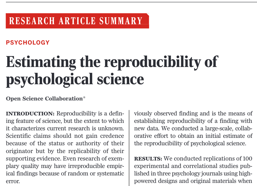
Summary
- reproducibility of 100 studies in psychological science from three high-ranking psychology journals
- 36% of the replications yielded significant findings
- compared to 97% of the original studies
- The mean effect size in the replications was approximately half the magnitude of the effects reported in the original studies
This is not limited to psychology
Why does this happens?
Journal of the Royal Statistical Society and American Statistical Association

Cargo cults

Original context

Richard Feynman
- Physicist
- Excellent professor
- Worked in the Manhattan Project at 25 years old
- Nobel Prize on Physics in 1965
Who do you want to be?


References
Erika Check Hayden, Weak statistical standards implicated in scientific irreproducibility Nature, 11 November 2013
Open Science Collaboration, Estimating the reproducibility of psychological science. Science 28 Aug 2015: Vol. 349, Issue 6251, aac4716 DOI: 10.1126/science.aac4716
Replications can cause distorted belief in scientific progress Behavioral and Brain Sciences, Volume 41, 2018, e122 DOI: https://doi.org/10.1017/S0140525X18000584. Published online by Cambridge University Press: 27 July 2018
References
Reproducibility of Scientific Results Stanford Encyclopedia of Philosophy
T.D. Stanley, Evan C. Carter and Hristos Doucouliagos What Meta-Analyses Reveal about the Replicability of Psychological Research Deakin Laboratory for the Meta-Analysis of Research, Working Paper, November 2017
Silas Boye Nissen, Tali Magidson, Kevin Gross, Carl T Bergstrom Research: Publication bias and the canonization of false facts eLife Dec 20, 2016;5:e21451 DOI: 10.7554/eLife.21451
Matrix
We study expressions like this
\[ \begin{aligned} y_1 & = x_{1,1}\, \beta_1 + x_{1,2}\, \beta_2\\ y_2 & = x_{2,1}\, \beta_1 + x_{2,2}\, \beta_2 \end{aligned} \]
we can do it again
\[ \begin{aligned} z_1 & = w_{1,1}\, y_1 + w_{1,2}\, y_2\\ z_2 & = w_{2,1}\, y_1 + w_{2,2}\, y_2 \end{aligned} \] We used \(x_{ij}\) for the coefficients of the first case, and \(w_{ij}\) for the second case.
Replacing the first equations in the second ones, we get
\[ \begin{aligned} z_1 & = w_{1,1}(x_{1,1}\, \beta_1+x_{1,2}\, \beta_2)+w_{1,2}(x_{2,1}\, \beta_1 + x_{2,2}\, \beta_2)\\ z_2 & = w_{2,1}(x_{1,1}\, \beta_1+x_{1,2}\, \beta_2)+w_{2,2}(x_{2,1}\, \beta_1 + x_{2,2}\, \beta_2) \end{aligned} \]
Let’s reorganize the terms
We get \[ \begin{aligned} z_1 & = (w_{1,1}x_{1,1}+w_{1,2}x_{2,1})\beta_1+(w_{1,1}x_{1,2}+w_{1,2}x_{2,2})\beta_2\\ z_2 & = (w_{2,1}x_{1,1}+w_{2,2}x_{2,1})\beta_1+(w_{2,1}x_{1,2}+w_{2,2}x_{2,2})\beta_2 \end{aligned} \] so we can go directly from \((\beta_1,\beta_2)\) to \((z_1,z_2)\) with the same kind of formula.
If we rewrite the last equations like this
\[ \begin{aligned} z_1 & = c_{1,1}\, \beta_1+ c_{1,2}\, \beta_2\\ z_2 & = c_{2,1}\, \beta_1+ c_{2,2}\, \beta_2 \end{aligned} \] we will have the following equivalences
values of \(c_{i,j}\)
\[ \begin{aligned} c_{1,1} & =w_{1,1}\, x_{1,1}+w_{1,2}\, x_{2,1} \\ c_{1,2} & =w_{1,1}\, x_{1,2}+w_{1,2}\, x_{2,2} \\ c_{2,1} & =w_{2,1}\, x_{1,1}+w_{2,2}\, x_{2,1} \\ c_{2,2} & =w_{2,1}\, x_{1,2}+w_{2,2}\, x_{2,2} \end{aligned} \]
This set of equivalences is usually abbreviated with the formula \[c_{i,j} = \sum_k w_{i,k} x_{k,j}\]
Simplifying the notation
There are so many numbers that is hard to follow what is exactly happening.
Fortunately, we can use the intrinsic structure of the equations to write them more clearly.
For example, in the equations
\[
\begin{aligned}
y_1 & = x_{1,1}\,\beta_1 + x_{1,2}\,\beta_2\\
y_2 & = x_{2,1}\,\beta_1 + x_{2,2}\,\beta_2
\end{aligned}
\] we can see that the first part of the right hand —between the
= and the + signs— is always multiplied by
\(\beta_1\),
and the second part —after the + sign— is always multiplied
by \(\beta_2\).
If this is always the case, we do not need to write
We neither need the + sign. Instead we can write \[
\begin{pmatrix}
y_1 \\ y_2
\end{pmatrix}
=
\begin{pmatrix}
x_{1,1} & x_{1,2}\\
x_{2,1} & x_{2,2}
\end{pmatrix}
\begin{pmatrix}
\beta_1 \\ \beta_2
\end{pmatrix}
\]
Using the same notation
We can therefore write the equations for \(z_1,z_2\) as \[ \begin{pmatrix} z_1 \\ z_2 \end{pmatrix} = \begin{pmatrix} w_{1,1} & w_{1,2}\\ w_{2,1} & w_{2,2} \end{pmatrix} \begin{pmatrix} y_1 \\ y_2 \end{pmatrix} \] and replacing \(y_1,y_2\), we have \[ \begin{pmatrix} z_1 \\ z_2 \end{pmatrix} = \begin{pmatrix} w_{1,1} & w_{1,2}\\ w_{2,1} & w_{2,2} \end{pmatrix} \begin{pmatrix} x_{1,1} & x_{1,2}\\ x_{2,1} & x_{2,2} \end{pmatrix} \begin{pmatrix} \beta_1 \\ \beta_2 \end{pmatrix} \] which is a formula that connects \(\beta_1,\beta_2\) and \(z_1,z_2\),
We also wrote \(z_1,z_2\), as
\[ \begin{pmatrix} z_1 \\ z_2 \end{pmatrix} = \begin{pmatrix} c_{1,1} & c_{1,2}\\ c_{2,1} & c_{2,2} \end{pmatrix} \begin{pmatrix} \beta_1 \\ \beta_2 \end{pmatrix} \]
Therefore, we are allowed to write \[ \begin{pmatrix} c_{1,1} & c_{1,2}\\ c_{2,1} & c_{2,2} \end{pmatrix} = \begin{pmatrix} w_{1,1} & w_{1,2}\\ w_{2,1} & w_{2,2} \end{pmatrix} \begin{pmatrix} x_{1,1} & x_{1,2}\\ x_{2,1} & x_{2,2} \end{pmatrix} \]
We can simplify the notation even more
Giving names to the matrices. Let’s call \[ \begin{aligned} \mathbf A & = \begin{pmatrix} x_{1,1} & x_{1,2}\\ x_{2,1} & x_{2,2} \end{pmatrix} \\ \mathbf B & = \begin{pmatrix} w_{1,1} & w_{1,2}\\ w_{2,1} & w_{2,2} \end{pmatrix}\\ \mathbf C & = \begin{pmatrix} c_{1,1} & c_{1,2}\\ c_{2,1} & c_{2,2} \end{pmatrix} \end{aligned} \] and now we can write \[\mathbf C =\mathbf B\mathbf A \]
Vectors and matrices
\[y= \begin{pmatrix} y_{1} \\ y_{2} \end{pmatrix} \]
Matrices are transformations
The matrix \(\mathbf X\) transforms the vector \(\mathbf \beta=(\beta_1, \beta_2)\) into the vector \(\mathbf y=(y_1, y_2)\) \[ \begin{aligned} y_1 & = x_{1,1}\, \beta_1 + x_{1,2}\, \beta_2\\ y_2 & = x_{2,1}\, \beta_1 + x_{2,2}\, \beta_2 \end{aligned} \] which can be written as \[ \begin{pmatrix} y_1 \\ y_2 \end{pmatrix} = \begin{pmatrix} x_{1,1} & x_{1,2}\\ x_{2,1} & x_{2,2} \end{pmatrix} \begin{pmatrix} \beta_1 \\ \beta_2 \end{pmatrix} \]
Using names for vectors and matrices
we get \[\mathbf y = \mathbf{X\beta}\]
Therefore, when we multiply a matrix \(\mathbf X\) with a column vector \(\mathbf \beta\), we get a new vector \(\mathbf y\) with the following values \[y_i = \sum_k x_{i,k} x_k\]
General matrix multiplication
You may have noticed that we did not specify the range of \(k\) in the multiplication formulas. This is intentional. The range is “whatever corresponds”. For the multiplication of two matrices, the condition is
the number of columns of the first matrix must be equal to the number of rows of the second matrix
Therefore, if \(\mathbf A\in\mathbb R^{m\times l}\) and \(\mathbf B\in\mathbb R^{l\times n}\) then \(\mathbf A\mathbf B\in\mathbb R^{m\times n}.\)
For the multiplication of a matrix with a vector
the condition is
number of columns of the matrix equal to number of rows of the vector
If \(\mathbf A\in\mathbb R^{m\times n}\) and \(\mathbf x\in\mathbb R^{n}\) then \(\mathbf A\mathbf x\in\mathbb R^{m}.\)
Here is the good idea
if we take the vectors in \(\mathbb R^{n}\) as matrices in \(\mathbb R^{n\times 1}\)—that is, if the vectors are one-column matrices— then matrix–vector multiplication is the same as matrix–matrix multiplication.
It is easy to see that rectangular matrices can be multiplied only in one way. The multiplication \[\mathbf A_{m\times_l}\mathbf B_{l\times n}\] is valid, but \[\mathbf B_{l\times n}\mathbf A_{m\times_l}\] is not, in general, unless \(n=m.\)
Square matrices
When we work with square matrices, then \(\mathbf A\mathbf B\) and \(\mathbf B\mathbf A\) are valid multiplications.
It is easy to see that, in general, \[\mathbf A\mathbf B\not=\mathbf B\mathbf A\]
Molecular Evolution
Mutation rate is not proportional to time
Multiple substitutions of the same base cannot be observed
GLMTVMNHMSMVDDPLVWATLPYKLFTSLDNIRWSLGAHNICFQNKFLANFFSLGQVLST
GVLVVPNHRSTLDDPLMWGVLPWSMLLRPRLMRWSLGAAELCFTNAVTSSMSSLAQVLAT
GVLVVPNHRSTLDDPLMWGTLPWSMLLRPRLMRWSLGAAELCFTNPVTSMMSSLAQVLAT
GLITVSNHQSCMDDPHLWGILKLRHIWNLKLMRWTPAAADICFTKELHSHFFSLGKCVPV
So we underestimate the divergence time
Blast hits for Taz1 (Saccharomyces cerevisiae, QHB12384.1) in RefSeq select proteins
probability of mutation
We know that \[ℙ(A,B)=ℙ(A)⋅ℙ(B|A)\] Therefore \[ℙ(B|A)=\frac{ℙ(A,B)}{ℙ(A)}\]
Here \(A\) is “initial amino acid is
Valine”
\(B\) is “new amino acid is
Leucine”
(or any other combination of amino acids)
Estimating short-term probabilities
By comparing highly-similar sequences, Margaret Dayhoff determined the frequencies of mutation for each pair of amino-acids in the short term.
This is a matrix, called PAM1 (“Point Accepted Mutations”), representing
\[ℙ(A\text{ at time }t, B\text{ at time }t+1)\]
We can write it as a matrix \[P_1 (A,B) = ℙ(A\text{ at time }t, B\text{ at time }t+1)\]
Dayhoff, Mo, and Rm Schwartz. “A Model of Evolutionary Change in Proteins.”. In Atlas of Protein Sequence and Structure. Washington, DC: National Biomedical Research Foundation, 1978. https://doi.org/10.1.1.145.4315.
Mutation probability
Let’s make the matrix of conditional probabilities \[ \begin{aligned} M_1(A,B)=&ℙ( B\text{ at time }t+1|A\text{ at time }t)\\ =& \frac{ℙ(A\text{ at time }t, B\text{ at time }t+1)}{ℙ(A\text{ at time }t)} \end{aligned} \]
We can build this matrix if we know \(ℙ(A\text{ at time }t)\)
We can find that probability by counting the frequency of each amino acid.
Calculating long-term evolution
\[ℙ(B\text{ at time }t+2|A\text{ at time }t)\]