Experiment
We have two samples (males and females), of size \(N\) each
We somehow know the variance \(σ^2\)
of each group
We calculate \(Z=(\bar{X}_f -
\bar{X}_m)/σ\) for our samples
This value \(Z\) follows a Normal
distribution (why?)
Under \(H_0\) the mean of \(Z\) is 0, but not under \(H_a\)
Evaluating the p-value
If \(H_0\) is true, \((\bar{X}_f - \bar{X}_m)\) follows a \(Normal(0, σ^2)\)
Therefore \(Z\) follows a \(Normal(0, 1)\)
In an experiment we get a fixed value \(z\)
The \(p\)-value is the probability
of getting the value \(z\) or more
extreme in our experiment \[ℙ(z ≥
\text{abs}(Z)|H_0, σ^2)\]
This is a two side test, since \(H_a\) is \(μ_f ≠
μ_m\)
We do not know the population variance
All we said before is true, but cannot be used directly
Because we do not know the population variance
Thus, we also ignore the population standard deviation
What can we do instead?
A solution
The solution is to use the standard deviation of the
sample
(do not confuse it with standard deviation of the sample
means)
But we have to pay a price: lower confidence
Sample variance instead of population variance
We need \(ℙ(\text{abs}(z) ≥
\text{abs}(Z)|H_0)\) but this time we do not know \(σ^2\)
Instead we have \(T=(\bar{X}_f -
\bar{X}_m)/S\), where \[S=\sqrt{\frac{\text{stdev}^2(X_f)+\text{stdev}^2(X_m)}{N}}\]
and \[\text{stdev}^2(X_f)=\frac{1}{N-1}\sum_{x∈ X_f}
(x-\bar{x})^2\]
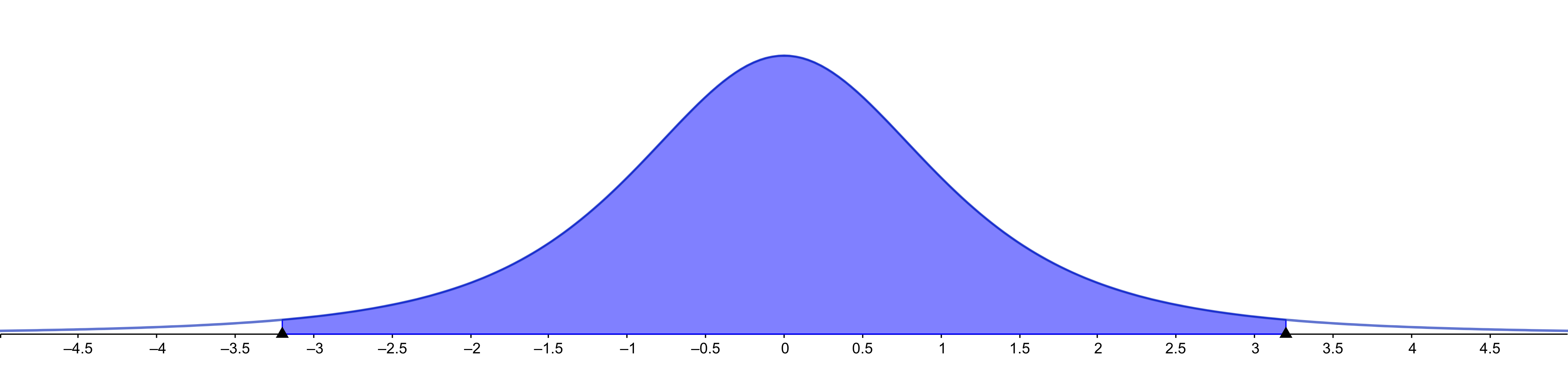
This is not Normal
The value \(T\) follows a Student’s
t-distribution
![]()
It is bell shaped, symmetric, but not Normal
Student’s t-distribution is wider than
Normal
![]()
Intervals are wider than Normal intervals
(but less than with Chebyshev)
Who was the Student?
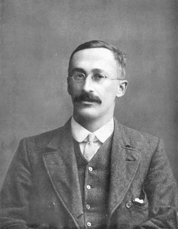
Published by William Sealy Gosset in Biometrika (1908)
He worked at the Guinness Brewery in Ireland
Studied small samples (the chemical properties of barley)
He called it “frequency distribution of standard deviations of
samples drawn from a normal population”
Story says that Guinness did not want their competitors to know this
quality control, so he used the pseudonym “Student”
It is a family of Student’s distributions
Here we use the sample standard deviation to approximate the
population standard deviation
As we have seen, if the sample is small, these two values may be
different
Thus, the Student’s distribution depends on the sample
size
More precisely, it depends on the degrees of freedom
Degrees of Freedom
The key idea is that the sample has \(N\) elements, but they are constrained by 1
value: the sample average
We say that we have \(N-1\)
degrees of freedom
![]()
Now it is not Normal
For the Normal distribution \[ℙ(\text{abs}(z) ≥ \text{abs}(Z) |H_0, σ)\]
is calculated as 2*(1-NORMSDIST(z))
For the Student’s t distribution \[ℙ(\text{abs}(t) ≥ \text{abs}(T) |H_0)\] is
calculated as 2*(1-T.DIST(t))
Finding Student’s confidence intervals
If we have 95% of population in the center, then we have 2.5% to the
left and 2.5% to the right
If the sample standard deviation is \(s\), the interval is \[[\bar{x} - k⋅s,\bar{x} + k⋅s]\]
We can find the \(k\) value if the
sample size is 5
T.INV(0.025, 5-1)
T.INV(0.975, 5-1)
\(k\) depends on
sample size
![]()
Summary
- Normal distributions are common in nature
- They happen when many things add together
- If the process is Normal, then the sample average is close to the
population average
- The confidence interval uses the t-Student distribution