Class 9: Sampling and population
Methodology of Scientific Research
Andrés Aravena, PhD
April 21, 2022
Example: cell counting
Hemocytometer
Each square is a sample. Volume is fixed. The cell count is an average of cell counts of some squares.
We want population cell density
We have a sample of cell densities
Different samples have different average

Bar plot

Representing the sample with a single value
Variance: Quality of representation
Standard Deviation
Standard Deviation is the “width” of population
We care about sd(x) because it tells us how close is the
mean to most of the population
It can be proved that always \[\Pr(\vert x_i-\bar{\mathbf x}\vert\geq k\cdot\text{sd}(\mathbf x))\leq 1/k^2\]
In other words, the probability that “the distance between the mean \(\bar{\mathbf x}\) and any element \(x_i\) is bigger than \(k\cdot\text{sd}(\mathbf x)\)” is less than \((1/k^2)\)
This is Chebyshev’s inequality
It is always valid, for any probability distribution
(Later we will see better rules valid only sometimes)
It can also be written as \[\Pr(\vert x_i-\bar{\mathbf x}\vert\leq k\cdot\text{sd}(\mathbf x))\geq 1-1/k^2\]
The probability that “the distance between the mean \(\bar{\mathbf x}\) and any element \(x_i\) is less than \(k\cdot\text{sd}(\mathbf x)\)” is greater than \(1-1/k^2\)
Some examples of Chebyshev’s inequality
Another way to understand the meaning of this theorem is \[\Pr(\bar{\mathbf x} -k\cdot\text{sd}(\mathbf x)\leq x_i \leq \bar{\mathbf x} +k\cdot\text{sd}(\mathbf x))\geq 1-1/k^2\] Replacing \(k\) for some values, we get
\[\begin{aligned} \Pr(\bar{\mathbf x} -1\cdot\text{sd}(\mathbf x)\leq x_i \leq \bar{\mathbf x} +1\cdot\text{sd}(\mathbf x))&\geq 1-1/1^2 = 0\\ \Pr(\bar{\mathbf x} -2\cdot\text{sd}(\mathbf x)\leq x_i \leq \bar{\mathbf x} +2\cdot\text{sd}(\mathbf x))&\geq 1-1/2^2 = 0.75\\ \Pr(\bar{\mathbf x} -3\cdot\text{sd}(\mathbf x)\leq x_i \leq \bar{\mathbf x} +3\cdot\text{sd}(\mathbf x))&\geq 1-1/3^2 = 0.889 \end{aligned}\]
From stats.libretexts.org
For any numerical data set
- at least 3/4 of the data lie within two standard deviations of the mean, that is, in the interval with endpoints \(\bar{\mathbf x}±2\cdot\text{sd}(\mathbf x)\)
- at least 8/9 of the data lie within three standard deviations of the mean, that is, in the interval with endpoints \(\bar{\mathbf x}±3\cdot\text{sd}(\mathbf x)\)
- at least \(1-1/k^2\) of the data lie within \(k\) standard deviations of the mean, that is, in the interval with endpoints \(\bar{\mathbf x}±k\cdot\text{sd}(\mathbf x),\) where \(k\) is any positive whole number greater than 1
The Empirical Rule and Chebyshev’s Theorem. (2021, January 11). Retrieved May 25, 2021, from https://stats.libretexts.org/@go/page/559
Example: the case of pop_HD
These values should be more than 0, 0.75 and 0.889
[1] 0.583[1] 1[1] 1Sampling
Simulating cell counting

Sample mean is a random variable

Bad news!
The sample average
changes every time
Moreover, it is often different from the population average
Sample average v/s size

Sample average v/s size

Average of smaller samples are more extreme
Good news
When the sample size is big,
the sample average is closer to
the population average
Variation depends on sample size

Log-log plot (for high density population)
plot(log(sd_sample_mean)~log(size))
model_HD <- lm(log(sd_sample_mean)~log(size))
lines(predict(model_HD)~log(size))
Linear model
(Intercept)   log(size)
      3.200      -0.516
\[\log(\text{sd_sample_mean}) = 3.2 + -0.516\cdot\log(\text{size})\] \[\begin{aligned}\text{sd_sample_mean} & = \exp(3.2) \cdot\text{size}^{-0.516}\\ & = 24.529\cdot\text{size}^{-0.516} \end{aligned}\]
Models for all populations
\[\text{sd_sample_mean} = A\cdot \text{size}^B\]
| A | B | std dev population | |
|---|---|---|---|
| pop_LD | 3.45 | -0.5261 | 3.188 |
| pop_MD | 9.455 | -0.5167 | 8.919 |
| pop_HD | 24.53 | -0.5158 | 23.14 |
Coefficient \(A\) is the standard
deviation of the population
Coefficient \(B\) is -0.5
What does this mean
If we know the population standard deviation, we can predict the sample standard deviation
\[\text{sd(sample mean)} = \frac{\text{sd(population)}}{\sqrt{\text{sample size}}}\]
Law of Large Numbers
Using Chebyshev formula, we know that, with high probability \[\vert \text{mean(sample)} -\text{mean(population)}\vert < k\cdot\frac{\text{sd(population)}}{\sqrt{\text{sample size}}}\]
Therefore the population average is inside the interval \[\text{mean(sample)} \pm k\cdot\frac{\text{sd(population)}}{\sqrt{\text{sample size}}}\] (probably)
How to know population standard deviation?
Remember that we do not know neither the population mean nor the population variance
So we do not know the population standard deviation 😕
In most cases we can use the sample standard deviation
Visually

Application
Answering scientific questions
Where are the cancers?
Highest kidney cancer rates in US (1980–1989) were in rural areas
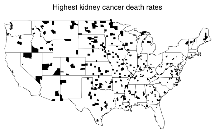
Highest rates of kidney cancer are in rural areas
Why? Maybe…
- the health care there is worse than in major cities
- High stress due to poverty
- are exposed to more harmful chemicals
- Drink Alcohol
- Smoke Tobacco
Lowest rates of kidney cancer are in rural areas
Why? Maybe…
- No air and water pollution.
- No stress
- Eat healthy foods
Something is wrong, of course. The rural lifestyle cannot explain both very high and very low incidence of kidney cancer.
Why smaller genes have extreme GC content

We will answer these question later
Some concepts
- Random variable
- number that depends on the outcome of a random process
- Average of population
- a fixed number, that we do not know and want to know
- Average of a sample
- a random variable, that we get from an experiment
Many things are averages
- concentration
- proportion
- density
- GC content
- frequency of events
What is the relationship between sample average and population average?
Can we learn the population average from the sample average?