Class 19: Normalization in RNAseq

Systems Biology

Andrés Aravena, PhD

December 28, 2021

Mapping reads to reference genome

There are several tools used to map reads to a genome

bwa
bowtie
bowtie2
hisat2

Each one has several options, that you can read in their manual

All of them produces SAM/BAM files

Why they may give different results

Count Normalization

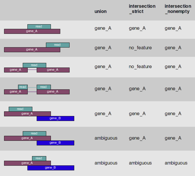
Using featureCounts (or similar) tool, we transform the SAM file into a matrix of counts

The element \(c_{ij}\) is the count of reads for gene \(i\) under library \(j\)

This value depends on

The gene expression
The gene length \(l_i\)
The number of reads in the library \(N_j\)

We care about the first one. The last one depends on technical issues

First idea: correct library effect

We can normalize the counts by the library size

The library size, i.e. the number of reads in the library, is \[N_j = \sum_i c_{ij}\]

So the relative number of reads is \[\frac{c_{ij}}{N_j}\]

These are small numbers

RNAseq libraries are large. They have millions of read

Thus, each \[\frac{c_{ij}}{N_j}\] is a very small number.

We scale them by \(10^6\) and get Reads Per Million \[\frac{c_{ij}⋅10^6}{N_j}\]

(same as we scale \(0.000004m\) to \(4μm\))

Larger genes have more reads

If the reads are taken randomly from each mRNA, then longer genes have higher probability of being sequenced

To correct that we divide by the gene length \(l_i\) \[\frac{c_{ij}⋅10^6}{N_j l_i}\]

Average gene length is around 1000bp

Again, this is a small number, so we scale by \(10^3\) and we get Reads Per Kilo per Million \[RPKM_{ij} = \frac{c_{ij}⋅10^9}{N_j l_i}\]

We can change the division order

It is easy to see that \[RPKM_{ij} = \frac{c_{ij}⋅10^6}{N_j} \frac{10^3}{l_i} = \frac{c_{ij}⋅10^3}{l_i} \frac{10^6}{N_j}\] so we can divide by the gene length first, and the library size later

Fragments instead of Reads

When we use paired-end sequencing, we typically get two reads for each fragment

But sometimes we get only one read

It makes sense to count fragments instead of reads

This is basically handled by the counting step

FPKM is the same formula as RPKM, but counting fragments instead of reads

Comparing libraries

We want to compare at least two libraries

The sum of all RPKM in library \(j_1\) is \[\sum_i RPKM_{i{j_1}} = \frac{10^9}{N_{j_1}}\sum_i \frac{c_{ij}}{l_i}\]

and, in general, this number is different from the sum for another library \(j_2\) \[\sum_i RPKM_{i{j_1}} ≠ \sum_i RPKM_{i{j_2}}\]

That is not good for statistical tests

Another way to normalize

To avoid this issue, we can normalize by the gene length before calculating totals

Let’s call \(Q_i\) to the sum of_gene-length-corrected_counts \[Q_j = \sum_i \frac{c_{ij}}{l_i}\]

Then Transcripts per Million for gene \(i\) in library \(j\) is \[TPM_{ij}=\frac{c_{ij}}{l_i⋅Q_j}\]

Now

Now we have \[\sum_i TPM_{ij}=\frac{1}{Q_j}\sum_i \frac{c_{ij}}{l_i}=1\]

Which one?

RPKM/FPKM are good for comparing between genes in the same library
TPM is better for comparing the same gene between libraries

DESeq2

This tool is based on a different statistical hypothesis

Instead of assuming log-normal distribution, it assumes a negative binomial distribution

Both distributions are similar, but it allows us to see the data from another point of view

In particular, it does not require normalization of counts

DESeq protocol

library(DESeq2)
read.counts <- read.table("GSE76307_transcript_counts.tsv")
head(read.counts)

          sw480_APC_1 sw480_APC_2 sw480_APC_3 sw480_CONTROL_1 sw480_CONTROL_2
NM_000014           1           1           3               1               2
NM_000015           1           0           0               0               2
NM_000016        1038        1126        1098            1285            1037
NM_000017         133         111         103             171             136
NM_000018        8699        8232        8364            8888            8426
NM_000019        2094        2070        1879            2645            2248
          sw480_CONTROL_3 sw480.1 sw480.2 sw480.3 cds_length gene_name
NM_000014               2       3       2       2       4653       A2M
NM_000015               1       1       3       1       1317      NAT2
NM_000016            1306    1022    1059    1057       2603     ACADM
NM_000017             174     143     147     125       1917     ACADS
NM_000018            9188   10982   10844   11450       2292    ACADVL
NM_000019            2775    2132    2164    2087       2134     ACAT1

Describe conditions of each sample

sample_info <- data.frame(
     condition=factor(rep(c("APC","CONTROL", "sw480"), each=3),
                      levels = c("CONTROL", "APC", "sw480")),
     row.names = colnames(read.counts[,1:9]))
sample_info

                condition
sw480_APC_1           APC
sw480_APC_2           APC
sw480_APC_3           APC
sw480_CONTROL_1   CONTROL
sw480_CONTROL_2   CONTROL
sw480_CONTROL_3   CONTROL
sw480.1             sw480
sw480.2             sw480
sw480.3             sw480

Pack everything in DESeq format

DESeq.ds <- DESeqDataSetFromMatrix( countData = read.counts[,1:9],
     colData = sample_info, design = ~ condition)
colData(DESeq.ds)

DataFrame with 9 rows and 1 column
                condition
                 <factor>
sw480_APC_1       APC    
sw480_APC_2       APC    
sw480_APC_3       APC    
sw480_CONTROL_1   CONTROL
sw480_CONTROL_2   CONTROL
sw480_CONTROL_3   CONTROL
sw480.1           sw480  
sw480.2           sw480  
sw480.3           sw480

rowData(DESeq.ds) # can be annotation data

DataFrame with 39276 rows and 0 columns

The data is there

counts(DESeq.ds) |> head()

          sw480_APC_1 sw480_APC_2 sw480_APC_3 sw480_CONTROL_1 sw480_CONTROL_2
NM_000014           1           1           3               1               2
NM_000015           1           0           0               0               2
NM_000016        1038        1126        1098            1285            1037
NM_000017         133         111         103             171             136
NM_000018        8699        8232        8364            8888            8426
NM_000019        2094        2070        1879            2645            2248
          sw480_CONTROL_3 sw480.1 sw480.2 sw480.3
NM_000014               2       3       2       2
NM_000015               1       1       3       1
NM_000016            1306    1022    1059    1057
NM_000017             174     143     147     125
NM_000018            9188   10982   10844   11450
NM_000019            2775    2132    2164    2087

Remove genes without any counts

DESeq.ds <- DESeq.ds[rowSums(counts(DESeq.ds)) > 0, ]

Now we verify that we did not lose any read

all(colSums(counts(DESeq.ds)) == colSums(read.counts[,1:9]))

[1] TRUE

Normalization by library

Estimate a factor to correct each library

DESeq.ds <- estimateSizeFactors(DESeq.ds)
sizeFactors(DESeq.ds)

    sw480_APC_1     sw480_APC_2     sw480_APC_3 sw480_CONTROL_1 sw480_CONTROL_2 
      1.0059487       0.9570850       0.9454599       1.0364710       0.9067061 
sw480_CONTROL_3         sw480.1         sw480.2         sw480.3 
      1.0709679       1.0344438       1.0359450       1.0370205

Normalized counts

It is just a factor of scale

counts.sf_normalized <- counts(DESeq.ds, normalized = TRUE)
plot(counts(DESeq.ds)[,1], counts.sf_normalized[,1], pch=".", log="xy")

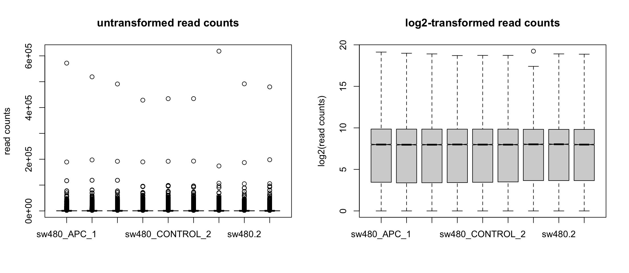
We can use logarithms

Let’s avoid log2(0) by adding a pseudo-count

log.norm.counts <- log2(counts.sf_normalized + 1)

DESeq does something different

DESeq.rlog <- rlog(DESeq.ds, blind = TRUE)
rlog.norm.counts <- assay(DESeq.rlog)

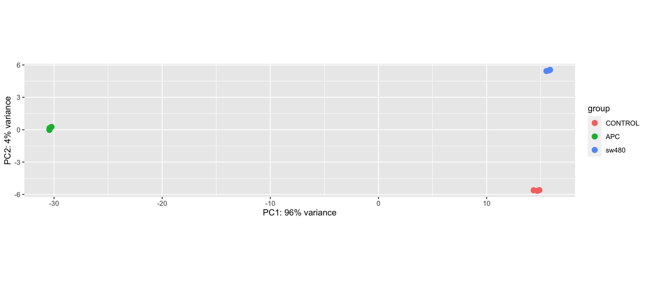
Comparing conditions

Principal Component Analysis

plotPCA(DESeq.rlog)

Let’s do the statistics

First, gene-wise dispersion estimates across all samples

DESeq.ds <- estimateDispersions(DESeq.ds)

gene-wise dispersion estimates

mean-dispersion relationship

final dispersion estimates

Then a t-test (assuming different variances)

DESeq.ds <- nbinomWaldTest(DESeq.ds)

Instead of `topTable`

results(DESeq.ds, independentFiltering = TRUE, alpha = 0.05) |> head()

log2 fold change (MLE): condition sw480 vs CONTROL 
Wald test p-value: condition sw480 vs CONTROL 
DataFrame with 6 rows and 6 columns
             baseMean log2FoldChange     lfcSE      stat      pvalue
            <numeric>      <numeric> <numeric> <numeric>   <numeric>
NM_000014    1.889930       0.433904 1.1851497  0.366118 7.14277e-01
NM_000015    0.995613       0.655316 1.6196758  0.404597 6.85774e-01
NM_000016 1111.347112      -0.251112 0.0621873 -4.038000 5.39089e-05
NM_000017  137.250467      -0.254684 0.1441359 -1.766968 7.72335e-02
NM_000018 9407.540815       0.281006 0.0384621  7.306038 2.75134e-13
NM_000019 2224.066114      -0.307231 0.0464157 -6.619114 3.61357e-11
                 padj
            <numeric>
NM_000014          NA
NM_000015          NA
NM_000016 2.67474e-04
NM_000017 1.56518e-01
NM_000018 4.40436e-12
NM_000019 4.61581e-10

Choosing another condition

results(DESeq.ds, contrast=c("condition", "APC", "CONTROL"),
     independentFiltering = TRUE, alpha = 0.05) |> head()

log2 fold change (MLE): condition APC vs CONTROL 
Wald test p-value: condition APC vs CONTROL 
DataFrame with 6 rows and 6 columns
             baseMean log2FoldChange     lfcSE       stat      pvalue
            <numeric>      <numeric> <numeric>  <numeric>   <numeric>
NM_000014    1.889930      0.0507329 1.2335629  0.0411271 9.67195e-01
NM_000015    0.995613     -1.4665320 1.8959505 -0.7735076 4.39222e-01
NM_000016 1111.347112     -0.0982781 0.0619814 -1.5856055 1.12829e-01
NM_000017  137.250467     -0.4190118 0.1475355 -2.8400750 4.51029e-03
NM_000018 9407.540815     -0.0189505 0.0387184 -0.4894445 6.24527e-01
NM_000019 2224.066114     -0.2909752 0.0466153 -6.2420551 4.31859e-10
                 padj
            <numeric>
NM_000014 9.83238e-01
NM_000015 5.45796e-01
NM_000016 1.73850e-01
NM_000017 9.33849e-03
NM_000018 7.18658e-01
NM_000019 1.76809e-09

Class 19: Normalization in RNAseq

Systems Biology

Andrés Aravena, PhD

December 28, 2021

Mapping reads to reference genome

Why they may give different results

Count Normalization

First idea: correct library effect

These are small numbers

Larger genes have more reads

Average gene length is around 1000bp

We can change the division order

Fragments instead of Reads

Comparing libraries

Another way to normalize

Now

Which one?

DESeq2

DESeq protocol

Describe conditions of each sample

Pack everything in DESeq format

The data is there

Remove genes without any counts

Normalization by library

Normalized counts

We can use logarithms

DESeq does something different

Comparing conditions

Principal Component Analysis

Let’s do the statistics

Instead of `topTable`

Choosing another condition

Big picture

Thanks for your attention

Class 19: Normalization in RNAseq

Systems Biology

Andrés Aravena, PhD

December 28, 2021

Mapping reads to reference genome

Why they may give different results

Count Normalization

First idea: correct library effect

These are small numbers

Larger genes have more reads

Average gene length is around 1000bp

We can change the division order

Fragments instead of Reads

Comparing libraries

Another way to normalize

Now

Which one?

DESeq2

DESeq protocol

Describe conditions of each sample

Pack everything in DESeq format

The data is there

Remove genes without any counts

Normalization by library

Normalized counts

We can use logarithms

DESeq does something different

Comparing conditions

Principal Component Analysis

Let’s do the statistics

Instead of topTable

Choosing another condition

Big picture

Thanks for your attention

Instead of `topTable`