Class 16: Analyzing Two-color Microarrays
Systems Biology
Andrés Aravena, PhD
December 17, 2021
Following the limma protocol
For today’s class we will follow the protocol for two-colors microarrays
- Define the experiment
- Read the hybridization data
- Normalize each slide internally
- Normalize between arrays
- Fit a linear model
- Evaluate statistical significance
Targets
It is recommended to start with a description of the experiments
We write a tab-separated file, indicating at least
                                 Filename    Cy3    Cy5
1       GSM3303967_Dcg2699_vs_WT_I.gpr.gz mutant     wt
2      GSM3303968_Dcg2699_vs_WT_II.gpr.gz mutant     wt
3 GSM3303969_Dcg2699_vs_WT_III_csw.gpr.gz     wt mutant
Reading the targets file
library(limma)
targets <- readTargets("targets.txt")
kable(targets)
| GSM3303967_Dcg2699_vs_WT_I.gpr.gz |
mutant |
wt |
| GSM3303968_Dcg2699_vs_WT_II.gpr.gz |
mutant |
wt |
| GSM3303969_Dcg2699_vs_WT_III_csw.gpr.gz |
wt |
mutant |
This example was taken from GSE117566 in NCBI GEO
Reading the arrays
RG <- read.maimages(targets$Filename, source = "genepix")
Read GSM3303967_Dcg2699_vs_WT_I.gpr.gz
Read GSM3303968_Dcg2699_vs_WT_II.gpr.gz
Read GSM3303969_Dcg2699_vs_WT_III_csw.gpr.gz
[1] "RGList"
attr(,"package")
[1] "limma"
[1] "R"       "G"       "Rb"      "Gb"      "targets" "genes"   "source"
[8] "printer"
[1] 45220 3
Genes
   Block Row Column              ID            Name
1      1   1      1 GE_BrightCorner GE_BrightCorner
2      1   1      2 GE_BrightCorner GE_BrightCorner
3      1   1      3      DarkCorner      DarkCorner
4      1   1      4      DarkCorner      DarkCorner
5      1   1      5      DarkCorner      DarkCorner
6      1   1      6      DarkCorner      DarkCorner
7      1   1      7      DarkCorner      DarkCorner
8      1   1      8      DarkCorner      DarkCorner
9      1   1      9      DarkCorner      DarkCorner
10     1   1     10      DarkCorner      DarkCorner
11     1   1     11      DarkCorner      DarkCorner
12     1   1     12      DarkCorner      DarkCorner
13     1   1     13      DarkCorner      DarkCorner
14     1   1     14      DarkCorner      DarkCorner
15     1   1     15      DarkCorner      DarkCorner
Comparing R and G channels
for(i in 1:3) plot(RG$R[,i], RG$G[,i])

Using Logarithms
for(i in 1:3) plot(log(RG$R[,i]), log(RG$G[,i]))

Looking at the slides
for(i in 1:3) imageplot(RG$R[,i], RG$printer)
for(i in 1:3) imageplot(RG$G[,i], RG$printer)

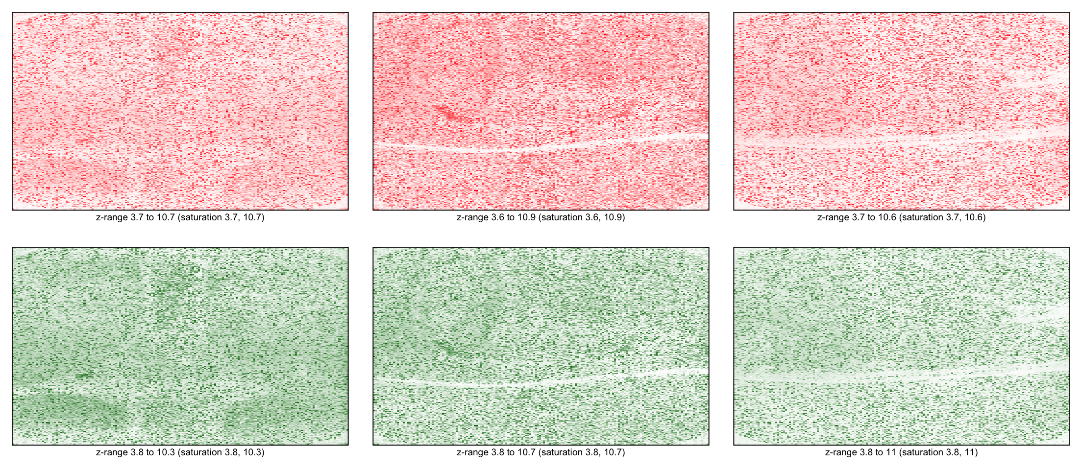
Using log
for(i in 1:3) imageplot(log(RG$R[,i]), RG$printer)
for(i in 1:3) imageplot(log(RG$G[,i]), RG$printer)
Background
for(i in 1:3) imageplot(log(RG$Rb[,i]), RG$printer)
for(i in 1:3) imageplot(log(RG$Gb[,i]), RG$printer)

Background correction
The easiest way to normalize is to subtract the background from the signal \[R_\text{corrected} = R - Rb\]
RG_corr <- backgroundCorrect(RG, method = "subtract")
class(RG_corr)
[1] "RGList"
attr(,"package")
[1] "limma"
[1] "R" "G" "targets" "genes" "source" "printer"
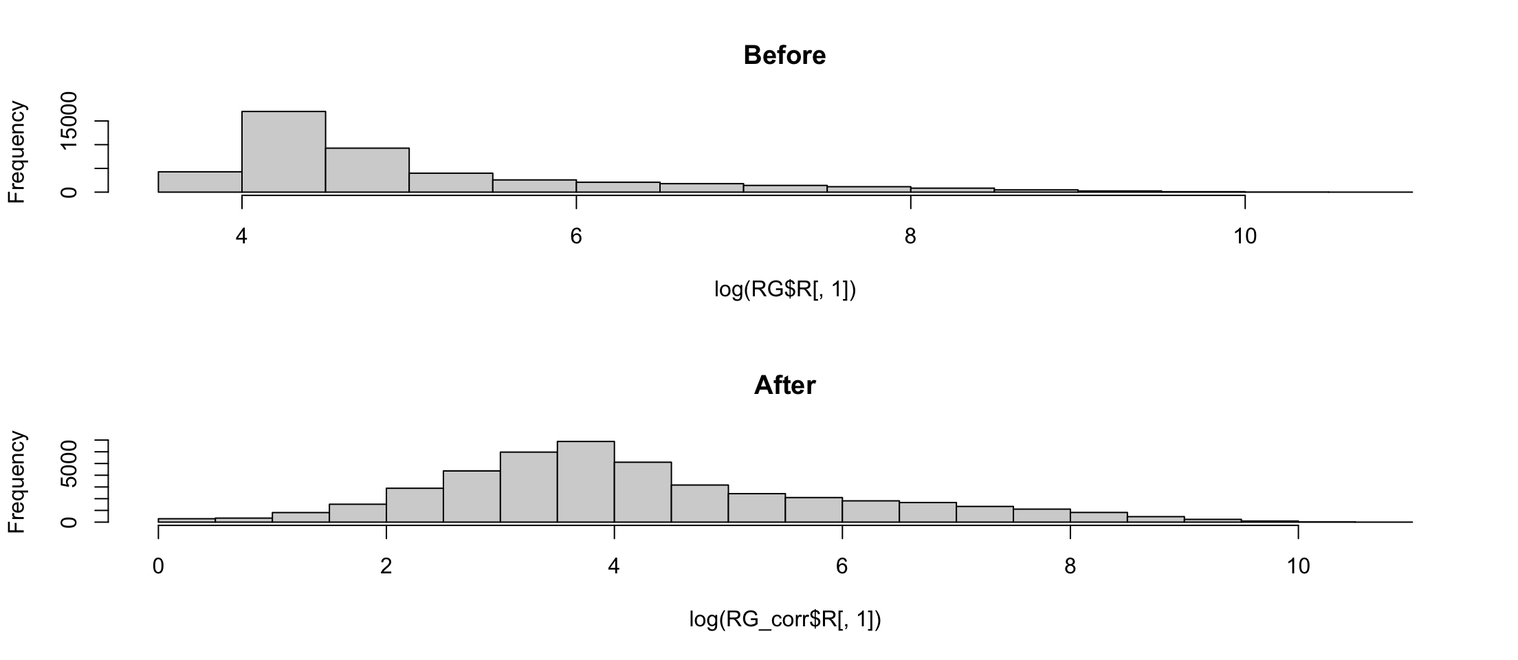
Histogram

There are negative numbers. Not good for logarithms
Histogram of log
Warning in log(RG_corr$R[, 1]): NaNs produced
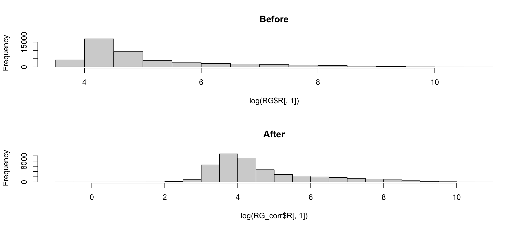
Avoiding negative values
A better correction requires a better model
RG_corr <- backgroundCorrect(RG, method = "normexp")
Array 1 corrected
Array 2 corrected
Array 3 corrected
Array 1 corrected
Array 2 corrected
Array 3 corrected
Normexp uses a model of background
Background corrected images
for(i in 1:3) imageplot(log(RG$R[,i]), RG$printer)
for(i in 1:3) imageplot(log(RG$G[,i]), RG$printer)

Comparing corrected
for(i in 1:3) plot(log(RG_corr$R[,i]), log(RG_corr$G[,i]))

Changing perspective
We care about the difference of expression \[M = \frac{\log(R)-\log(G)}{2}\]
For symmetry, we also keep the average expression \[ A = \frac{\log(R)+\log(G)}{2}\]
MA plot
for(i in 1:3) plotMA(RG_corr, array=i)

Correcting banana shape
MA <- normalizeWithinArrays(RG_corr, method="loess")
for(i in 1:3) plotMA(MA, array=i)

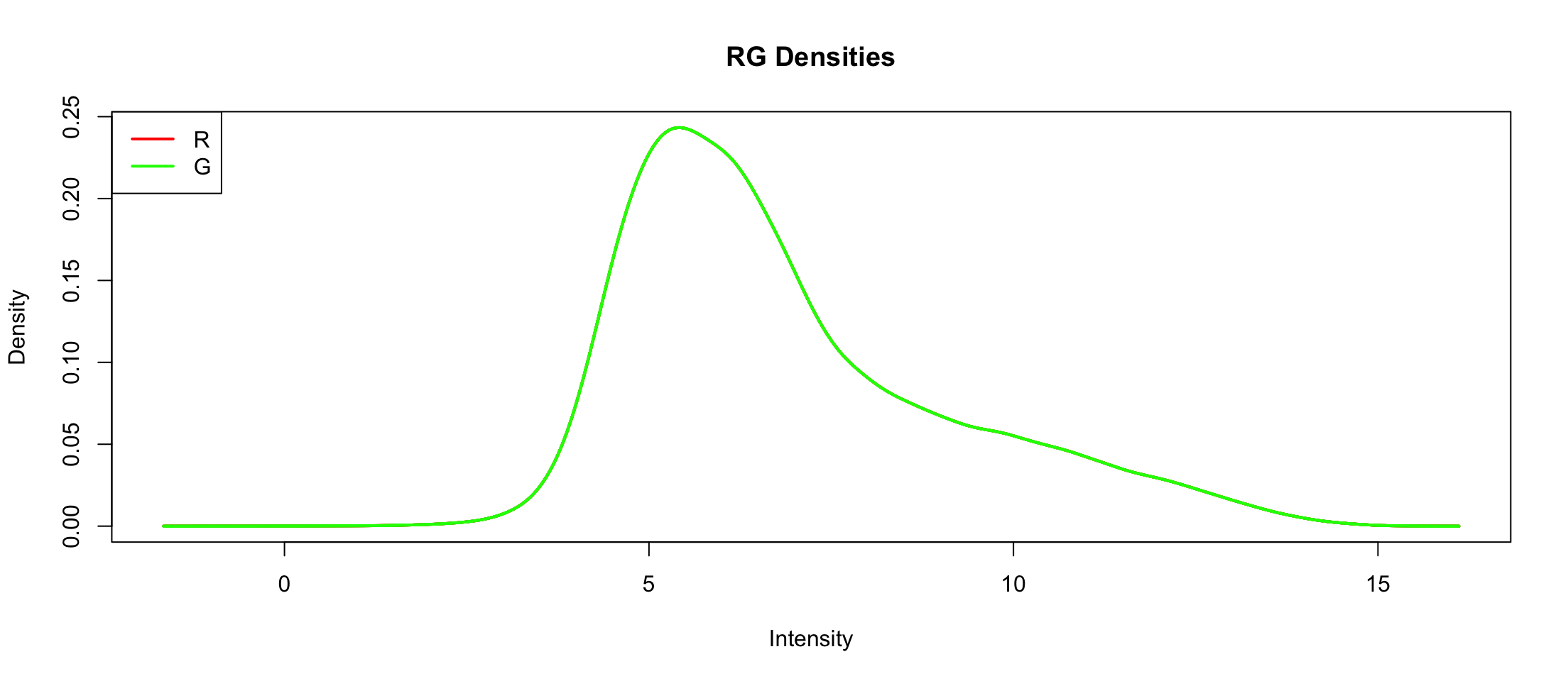
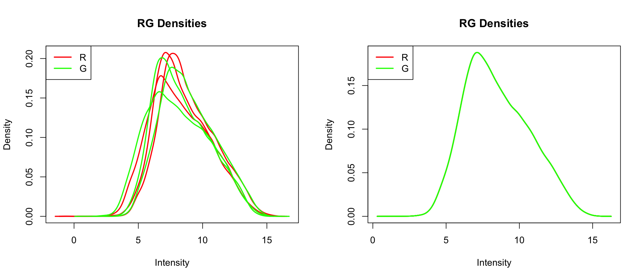
Comparing densities
Think of these as softened histograms
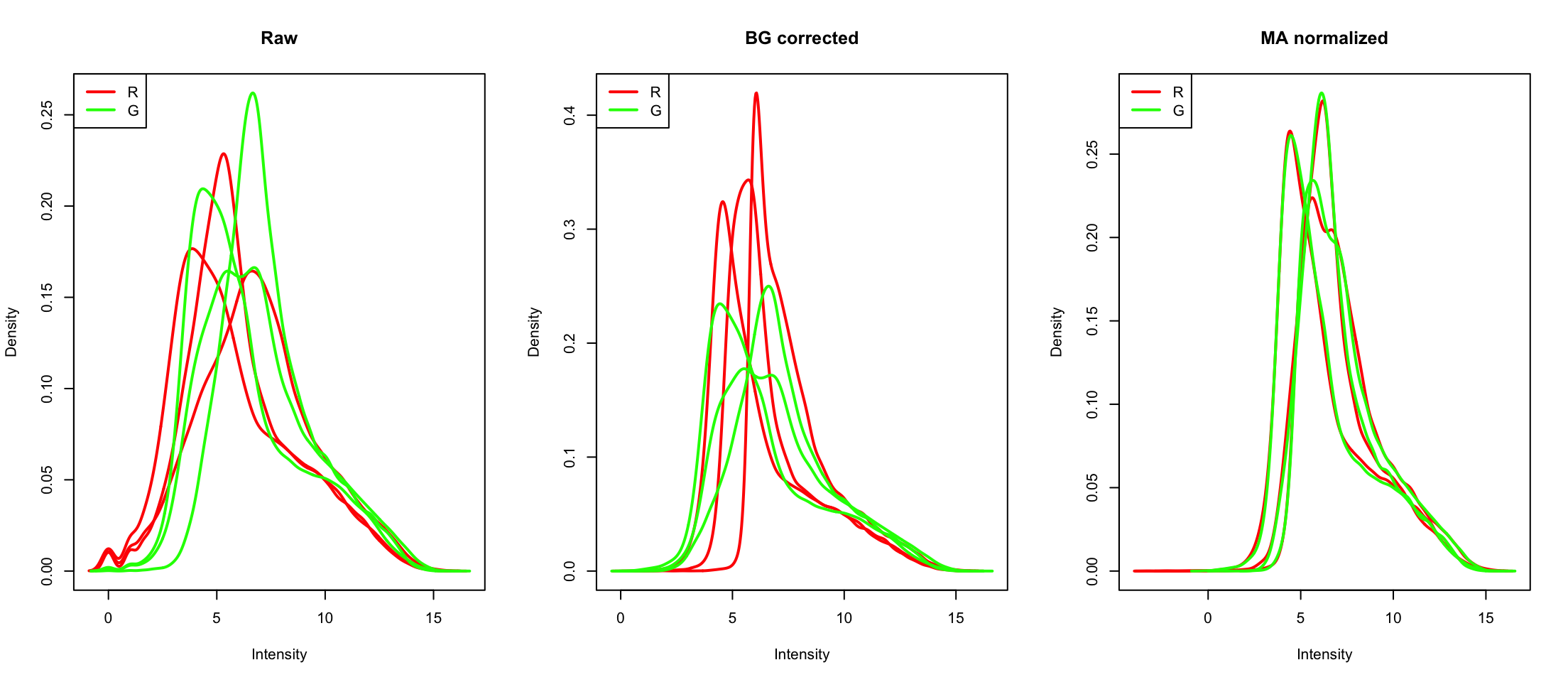
Between array normalization
MA.q <- normalizeBetweenArrays(MA, method = "quantile")
plotDensities(MA.q)
Let’s drop control spots
gal <- readGAL("GPL16989_Genepix_GAL_4plex_Design_041487.gal.gz")
# num_replicas <- table(MA$genes$ID)
# controls <- names(num_replicas)[num_replicas>=10]
MA <- MA[gal$ControlType == "false", ]
MA <- MA[MA$genes$ID != "EMPTY", ]
MA.q <- normalizeBetweenArrays(MA, method = "quantile")
Now we are ready to analyze
First, simplify gene description
There are many columns that we do not need anymore
Let’s drop them
MA.q$genes$Block <- NULL
MA.q$genes$Row <- NULL
MA.q$genes$Column <- NULL
MA.q$genes$ID <- NULL
This will simplify the presentation of results later
We can build a model matrix from targets
design <- modelMatrix(targets, ref = "wt")
Found unique target names:
 mutant wt
     mutant
[1,]     -1
[2,]     -1
[3,]      1
Now we fit it
fit <- lmFit(MA.q, design)
hist(fit$Amean)

Filter out the un-expressed spots
fit <- fit[fit$Amean>5, ]
topTable(eBayes(fit))
               Name     logFC   AveExpr         t      P.Value    adj.P.Val
1039         cg2071  5.428600  9.440261  26.03824 1.025257e-10 2.056051e-06
24758 TOCGc27704421 -5.412790 10.218971 -20.27835 1.277049e-09 1.109858e-05
42170        cg1299 -3.877140 10.355572 -18.36246 3.450906e-09 1.109858e-05
25823        cg1883 -3.955607 11.980194 -18.31029 3.550412e-09 1.109858e-05
18653        cg1881 -4.016262 11.966937 -18.00908 4.189938e-09 1.109858e-05
33607        cg1881 -3.851484 10.706278 -17.97686 4.265475e-09 1.109858e-05
7177         cg1883 -4.016393 11.083149 -17.57707 5.338004e-09 1.109858e-05
28545        cg1299 -3.878424 10.628074 -17.57305 5.350168e-09 1.109858e-05
37305        cg1884 -3.775995 10.826130 -17.54943 5.422361e-09 1.109858e-05
117          cg1881 -4.023286 12.212845 -17.48055 5.639087e-09 1.109858e-05
             B
1039  13.50041
24758 11.84673
42170 11.10935
25823 11.08761
18653 10.96019
33607 10.94637
7177  10.77173
28545 10.76995
37305 10.75944
117   10.72868