Class 15: Practice with Interaction Graphs

Systems Biology

Andrés Aravena, PhD

December 14, 2021

An example of microarray analysis

This is Atakan’s thesis work

We start with a description of the experiments

It is an Excel table, which we export as tab-separated file and read it in R

ff <- read.delim("intermittent_sdrf.tsv")
dim(ff)

[1] 81 10

We get a data frame with 81 rows and 10 columns

Let’s see the content

head(ff)

  individual     organism diet age..week. organism.part material.type  label
1        T95 Mus musculus   AL      49/50         Brain organism part biotin
2        T96 Mus musculus   AL      49/50         Brain organism part biotin
3       T207 Mus musculus   AL      49/50         Brain organism part biotin
4       T106 Mus musculus  CCR      49/50         Brain organism part biotin
5       T184 Mus musculus  CCR      49/50         Brain organism part biotin
6       T185 Mus musculus  CCR      49/50         Brain organism part biotin
  array.design              array.data.file
1    miRNA-4_0   Brain/AL_T95_Brain_w50.CEL
2    miRNA-4_0   Brain/AL_T96_Brain_w50.CEL
3    miRNA-4_0  Brain/AL_T207_Brain_w50.CEL
4    miRNA-4_0 Brain/CCR_T106_Brain_w50.CEL
5    miRNA-4_0 Brain/CCR_T184_brain_w50.CEL
6    miRNA-4_0 Brain/CCR_T185_Brain_w50.CEL
                               array.data.path
1   ~/CR-miRNA/Data/Brain/AL_T95_Brain_w50.CEL
2   ~/CR-miRNA/Data/Brain/AL_T96_Brain_w50.CEL
3  ~/CR-miRNA/Data/Brain/AL_T207_Brain_w50.CEL
4 ~/CR-miRNA/Data/Brain/CCR_T106_Brain_w50.CEL
5 ~/CR-miRNA/Data/Brain/CCR_T184_brain_w50.CEL
6 ~/CR-miRNA/Data/Brain/CCR_T185_Brain_w50.CEL

They used two platforms

The microarray slides changed during the experiments

table(ff$array.design)


miRNA-4_0 miRNA-4_1 
       12        69

That will make the analysis more complicated

For today we will use only one platforms

ff <- subset(ff, array.design == "miRNA-4_1")

How to read array data

There are several libraries for different platforms

We will see them later

For this data we use two libraries

library(oligo)
library(pd.mirna.4.1)

The last library has the description of the microarray probes

Reading the data

raw <- read.celfiles(ff$array.data.file)

Reading in : Brain/AL_T3_Brain_w80.ga.cel
Reading in : Brain/AL_T67_Brain_w80.ga.cel
Reading in : Brain/AL_T123_Brain_w80.ga.cel
Reading in : Brain/CCR_T33_Brain_w80.ga.cel
Reading in : Brain/CCR_T38_Brain_w80.ga.cel
Reading in : Brain/CCR_T125_Brain_w80.ga.cel
Reading in : Brain/ICRR_T137_Brain_w80.ga.cel
Reading in : Brain/ICRR_T70_Brain_w80.ga.cel
Reading in : Brain/ICRR_T22_Brain_w80.ga.cel
Reading in : Brain/ICRRF_T117_Brain_w80.ga.cel
Reading in : Brain/ICRRF_T116_Brain_w80.ga.cel
Reading in : Brain/ICRRF_T25_Brain_w80.ga.cel
Reading in : Blood/AL_T95_blood_w50.ga.cel
Reading in : Blood/AL_T96_blood_w50.ga.cel
Reading in : Blood/AL_T97_blood_w50.ga.cel
Reading in : Blood/CCR_T94_blood_w50.ga.cel
Reading in : Blood/CCR_T106_blood_w50.ga.cel
Reading in : Blood/CCR_T107_blood_w50.ga.cel
Reading in : Blood/ICRR_T79_blood_w50.ga.cel
Reading in : Blood/ICRR_T196_blood_w50.ga.cel
Reading in : Blood/ICRR_T197_blood_w50.ga.cel
Reading in : Blood/ICRRF_T76_blood_w50.ga.cel
Reading in : Blood/ICRRF_T111_blood_w50.ga.cel
Reading in : Blood/ICRRF_T223_blood_w50.ga.cel
Reading in : Blood/AL_T66_Blood_w80.ga.cel
Reading in : Blood/AL_T67_Blood_w80.ga.cel
Reading in : Blood/AL_T123_Blood_w80.ga.cel
Reading in : Blood/CCR_T38_Blood_w80.ga.cel
Reading in : Blood/CCR_T125_Blood_w80.ga.cel
Reading in : Blood/CCR_T126_Blood_w80.ga.cel
Reading in : Blood/ICRR_T70_Blood_w80.ga.cel
Reading in : Blood/ICRR_T137_Blood_w80.ga.cel
Reading in : Blood/ICRR_T138_Blood_w80.ga.cel
Reading in : Blood/ICRRF_T116_Blood_w80.ga.cel
Reading in : Blood/ICRRF_T117_Blood_w80.ga.cel
Reading in : Blood/ICRRF_T129_Blood_w80.ga.cel
Reading in : MFP/AL_T95_MFP_w50.ga.cel
Reading in : MFP/AL_T96_MFP_w50.ga.cel
Reading in : MFP/AL_T97_MFP_w50.ga.cel
Reading in : MFP/CCR_T94_MFP_w50.ga.cel
Reading in : MFP/CCR_T106_MFP_w50.ga.cel
Reading in : MFP/CCR_T107_MFP_w50.ga.cel
Reading in : MFP/ICRR_T130_MFP_w50.ga.cel
Reading in : MFP/ICRR_T133_MFP_w50.ga.cel
Reading in : MFP/ICRR_T134_MFP_w50.ga.cel
Reading in : MFP/ICRRF_T76_MFP_w50.ga.cel
Reading in : MFP/ICRRF_T77_MFP_w50.ga.cel
Reading in : MFP/ICRRF_T110_MFP_w50.ga.cel
Reading in : MFP/AL_T1_MFP_w80.ga.cel
Reading in : MFP/AL_T3_MFP_w80.ga.cel
Reading in : MFP/AL_T123_MFP_w80.ga.cel
Reading in : MFP/CCR_T33_MFP_w80.ga.cel
Reading in : MFP/CCR_T34_MFP_w80.ga.cel
Reading in : MFP/CCR_T37_MFP_w80.ga.cel
Reading in : MFP/ICRR_T20_MFP_w80.ga.cel
Reading in : MFP/ICRR_T44_MFP_w80.ga.cel
Reading in : MFP/ICRR_T71_MFP_w80.ga.cel
Reading in : MFP/ICRRF_T25_MFP_w80.ga.cel
Reading in : MFP/ICRRF_T116_MFP_w80.ga.cel
Reading in : MFP/ICRRF_T117_MFP_w80.ga.cel
Reading in : Brain/BASELINE_T233_Brain.ga.cel
Reading in : Brain/BASELINE_T234_Brain.ga.cel
Reading in : Brain/BASELINE_T242_Brain.ga.cel
Reading in : Blood/BASELINE_T234_blood.ga.cel
Reading in : Blood/BASELINE_T242_blood.ga.cel
Reading in : Blood/BASELINE_T251_blood.ga.cel
Reading in : MFP/BASELINE_T190_MFP.ga.cel
Reading in : MFP/BASELINE_T193_MFP.ga.cel
Reading in : MFP/BASELINE_T242_MFP.ga.cel

Normalization

We got a structure with dimensions

dim(raw)

Features  Samples 
  292681       69

Now we normalize it using functions from limma

library(limma)
eset <- rma(raw)
dim(eset)

Background correcting
Normalizing
Calculating Expression

Features  Samples 
   36353       69

These are S4 objects, different from typical R objects

We reduced from

Taking just the expression

We only need the expression matrix

norm.Data <- exprs(eset)
dim(norm.Data)

[1] 36353    69

This is a regular R matrix object

We reduced from 292681 to 36353 rows

Take a look

norm.Data[1:15, 1:2]

             AL_T3_Brain_w80.ga.cel AL_T67_Brain_w80.ga.cel
14q0_st                   0.3875505               0.3659802
14qI-1_st                 0.4611885               0.3843568
14qI-1_x_st               0.4611885               0.4297402
14qI-2_st                 0.4308127               0.4297402
14qI-3_x_st               0.5527731               0.3664233
14qI-4_st                 0.6316946               0.6469497
14qI-4_x_st               0.4580708               0.4804409
14qI-5_st                 0.5552395               0.5970109
14qI-6_st                -0.0346034               0.2649506
14qI-7_st                 0.8116030               0.5584780
14qI-8_st                 0.6690536               0.6415562
14qI-8_x_st               0.6538301               0.5694803
14qI-9_x_st               0.2490384               0.5425702
14qII-1_st                0.5560365               0.7858593
14qII-1_x_st              0.5590283               0.6877286

Keep only mouse miRNA

We want to use only relevant data

The miRNA description is in another file

annot <- read.csv("miRNA-4_1-st-v1.annotations.20160922.csv", comment = "#")
annot |> subset(Species.Scientific.Name=="Mus musculus") |>
         subset(pattern=str_starts("MIMAT")) -> mouse
mouse.data <- norm.Data[mouse$Probe.Set.Name, ]
dim(mouse.data)

[1] 3163   69

Condition for each sample

In this case each column name includes the condition

condition <- as.factor(stringr::str_remove(ff$diet,"-"))
condition

 [1] AL       AL       AL       CCR      CCR      CCR      ICRR     ICRR    
 [9] ICRR     ICRRF    ICRRF    ICRRF    AL       AL       AL       CCR     
[17] CCR      CCR      ICRR     ICRR     ICRR     ICRRF    ICRRF    ICRRF   
[25] AL       AL       AL       CCR      CCR      CCR      ICRR     ICRR    
[33] ICRR     ICRRF    ICRRF    ICRRF    AL       AL       AL       CCR     
[41] CCR      CCR      ICRR     ICRR     ICRR     ICRRF    ICRRF    ICRRF   
[49] AL       AL       AL       CCR      CCR      CCR      ICRR     ICRR    
[57] ICRR     ICRRF    ICRRF    ICRRF    BASELINE BASELINE BASELINE BASELINE
[65] BASELINE BASELINE BASELINE BASELINE BASELINE
Levels: AL BASELINE CCR ICRR ICRRF

Fitting the linear model

With the description of condition, we build a design matrix

design <- model.matrix(~ condition + 0)
colnames(design) <- levels(condition)
design

   AL BASELINE CCR ICRR ICRRF
1   1        0   0    0     0
2   1        0   0    0     0
3   1        0   0    0     0
4   0        0   1    0     0
5   0        0   1    0     0
6   0        0   1    0     0
7   0        0   0    1     0
8   0        0   0    1     0
9   0        0   0    1     0
10  0        0   0    0     1
11  0        0   0    0     1
12  0        0   0    0     1
13  1        0   0    0     0
14  1        0   0    0     0
15  1        0   0    0     0
16  0        0   1    0     0
17  0        0   1    0     0
18  0        0   1    0     0
19  0        0   0    1     0
20  0        0   0    1     0
21  0        0   0    1     0
22  0        0   0    0     1
23  0        0   0    0     1
24  0        0   0    0     1
25  1        0   0    0     0
26  1        0   0    0     0
27  1        0   0    0     0
28  0        0   1    0     0
29  0        0   1    0     0
30  0        0   1    0     0
31  0        0   0    1     0
32  0        0   0    1     0
33  0        0   0    1     0
34  0        0   0    0     1
35  0        0   0    0     1
36  0        0   0    0     1
37  1        0   0    0     0
38  1        0   0    0     0
39  1        0   0    0     0
40  0        0   1    0     0
41  0        0   1    0     0
42  0        0   1    0     0
43  0        0   0    1     0
44  0        0   0    1     0
45  0        0   0    1     0
46  0        0   0    0     1
47  0        0   0    0     1
48  0        0   0    0     1
49  1        0   0    0     0
50  1        0   0    0     0
51  1        0   0    0     0
52  0        0   1    0     0
53  0        0   1    0     0
54  0        0   1    0     0
55  0        0   0    1     0
56  0        0   0    1     0
57  0        0   0    1     0
58  0        0   0    0     1
59  0        0   0    0     1
60  0        0   0    0     1
61  0        1   0    0     0
62  0        1   0    0     0
63  0        1   0    0     0
64  0        1   0    0     0
65  0        1   0    0     0
66  0        1   0    0     0
67  0        1   0    0     0
68  0        1   0    0     0
69  0        1   0    0     0
attr(,"assign")
[1] 1 1 1 1 1
attr(,"contrasts")
attr(,"contrasts")$condition
[1] "contr.treatment"

Making contrasts

contrast.matrix <- makeContrasts(
    CvsA = CCR - AL,
    RvsA = ICRR - AL,
    RFvsA = ICRRF - AL,
    RvsC = ICRR - CCR,
    RFvsC = ICRRF - CCR,
    RvsRF = ICRR - ICRRF,
    levels = design
)

Fitting the model

fit <- lmFit(mouse.data, design)
fit.eb <- eBayes(contrasts.fit(fit, contrast.matrix))

Evaluating p-values

topTable(fit.eb) |> round(2)

                 CvsA  RvsA RFvsA  RvsC RFvsC RvsRF AveExpr    F P.Value
MIMAT0014941_st -0.22 -0.27  0.16 -0.05  0.38 -0.43    0.66 8.04    0.00
MI0009961_st     0.19  0.14  0.39 -0.06  0.20 -0.25    1.50 4.89    0.00
MI0022894_st     0.00  0.09  0.28  0.09  0.28 -0.19    0.87 4.87    0.00
MI0004300_st    -0.09  0.20 -0.09  0.29  0.00  0.29    0.82 4.30    0.01
MI0000560_st     0.01  0.11  0.34  0.09  0.33 -0.23    0.99 4.24    0.01
MIMAT0014950_st -0.04  0.10  0.22  0.14  0.25 -0.12    0.83 4.00    0.01
MI0022778_st    -0.04 -0.05  0.11 -0.02  0.15 -0.17    0.55 3.99    0.01
MIMAT0014822_st -0.14  0.23  0.01  0.37  0.14  0.22    0.76 3.88    0.01
MI0022921_st     0.01 -0.05  0.21 -0.06  0.20 -0.26    0.74 3.83    0.01
MIMAT0014838_st -0.12 -0.07  0.12  0.05  0.25 -0.20    0.43 3.82    0.01
                adj.P.Val
MIMAT0014941_st      0.39
MI0009961_st         1.00
MI0022894_st         1.00
MI0004300_st         1.00
MI0000560_st         1.00
MIMAT0014950_st      1.00
MI0022778_st         1.00
MIMAT0014822_st      1.00
MI0022921_st         1.00
MIMAT0014838_st      1.00

(in this example the p-values are bad, but anyway)

Experimental covariance

The last 4 columns are not differential expression values, so we drop them

top <- topTable(fit.eb, number = 10)
num_samples <- ncol(top)-4
top <- top[, 1:num_samples]

Now we calculate the covariance between the rows, so we transpose top

covar <- cov(t(top))

Using glasso

library(glasso)
ans <- glasso(covar, rho=0.02, nobs=num_samples)
ans$wi |> round(2)

       [,1]  [,2]  [,3]  [,4]  [,5]  [,6]  [,7]  [,8]  [,9] [,10]
 [1,] 16.00 -0.77 -4.55  0.67 -4.58 -4.14 -4.03  0.00 -4.38 -6.30
 [2,] -0.77 17.29 -1.87  3.84 -3.31  0.00  0.00  0.82 -3.23  0.00
 [3,] -4.55 -1.87 23.50  0.00 -3.09  0.00  0.00  0.00 -0.56  0.00
 [4,]  0.67  3.84  0.00 20.81  0.00  0.00  0.00 -3.18  0.58  0.00
 [5,] -4.58 -3.31 -3.09  0.00 20.76 -1.44  0.00  0.00 -2.10 -1.03
 [6,] -4.14  0.00  0.00  0.00 -1.44 26.80  0.00  0.00  0.00  0.00
 [7,] -4.03  0.00  0.00  0.00  0.00  0.00 31.51  0.00  0.00  0.00
 [8,]  0.00  0.82  0.00 -3.18  0.00  0.00  0.00 19.69  0.00  0.00
 [9,] -4.38 -3.23 -0.56  0.58 -2.10  0.00  0.00  0.00 23.59  0.00
[10,] -6.30  0.00  0.00  0.00 -1.03  0.00  0.00  0.00  0.00 25.06

We observe that the pseudoinverse has many zeros, as expected

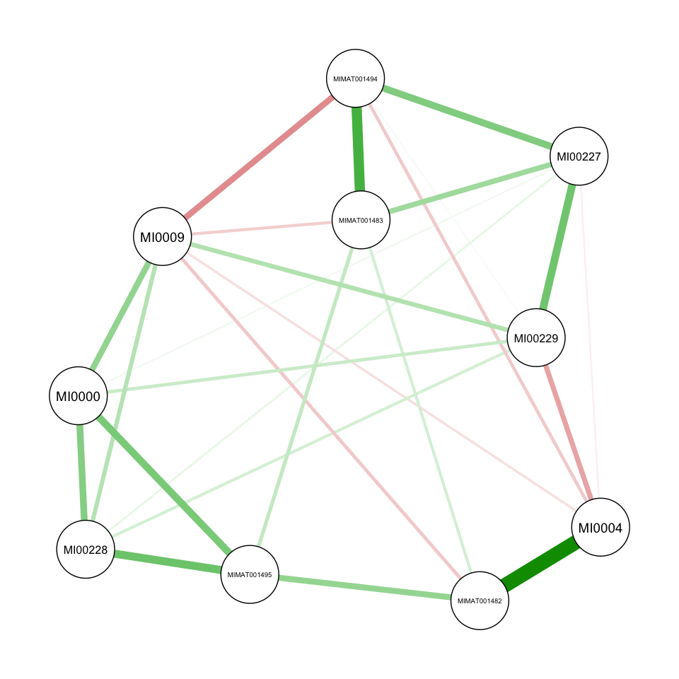
Graphical view

library(qgraph)
qgraph(ans, layout = "spring")

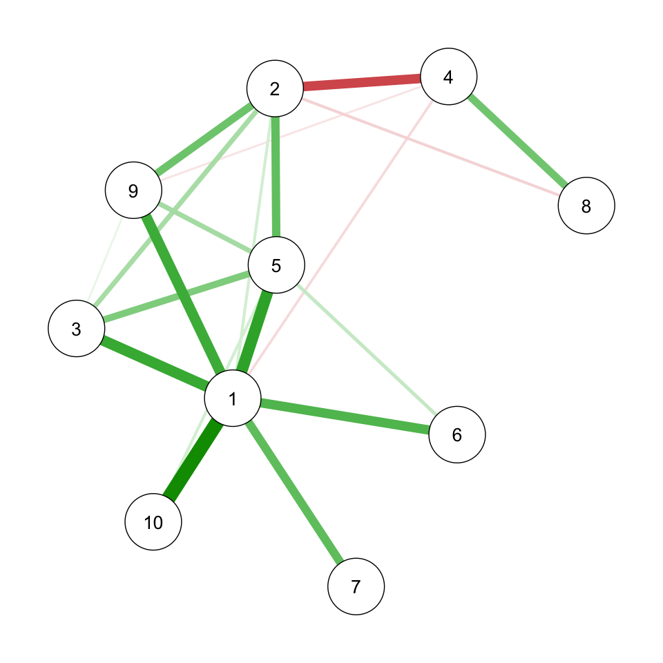
Optimal lambda/rho

best.ans <- EBICglasso(covar, num_samples, checkPD = FALSE)
qgraph(best.ans, layout = "spring")