Class 14: Interaction Graphs
Systems Biology
Andrés Aravena, PhD
December 07, 2021
Genes work in teams
We would like to know how genes/proteins/molecules interact
These interactions can be described with a network
So we would like to find the network that represent the interactions
At first, we want to know who interacts with who
Transcriptional regulation networks
Several parts: some genes encode transcription factors, which can bind to DNA
We simplify to a directed bipartite network: genes and binding sites
We can predict if a gene encodes a transcription factor
We can predict if a site is a binding site
But we need experiments to see which transcription factor binds to which sites
Interaction networks
Metabolic and transcriptional networks are very important, and we need several classes to study them
Today we begin with a simpler problem: gene interaction networks
These will be undirected non-bipartite networks
They may be later extended to a directed network with more attributes
What is interaction?
First idea: Correlation
It is a square matrix, so we can see it as an adjacency matrix
Thus, we can draw a network
What is the network?

Depending on how we define “significant correlation”, we have more or less edges
Not too small, not too big

If nothing is connected to nothing, we do not learn anything
The same happens if everything is connected to everything
Three strategies
Thresholding
Pruning
Regularization
Defining a threshold
Remember that we observe the sample correlation, which is usually different from the real correlation
Sample correlation may be non-zero even if the real correlation is zero
We can use a statistical test to decide which correlations are significant
This test defines a threshold, which depends on the number of nodes
Pruning

Even after thresholding, we often have spurious links
If A is correlated with B, and B is correlated with C, then there will be a small (but significant) correlation between A and C
One pruning strategy is to drop the “weakest link” of every triangle
Pruning cycles

Another strategy is to discard the “weakest link” in every cycle
This results in a network with the shape of a tree
More specifically, we get a Spanning Tree
Comparison
![]()
To do better we need to understand what is correlation
Assuming expression follows is Normal

Expression has a random component
Genes may not be independent
Plotting both values shows a pattern
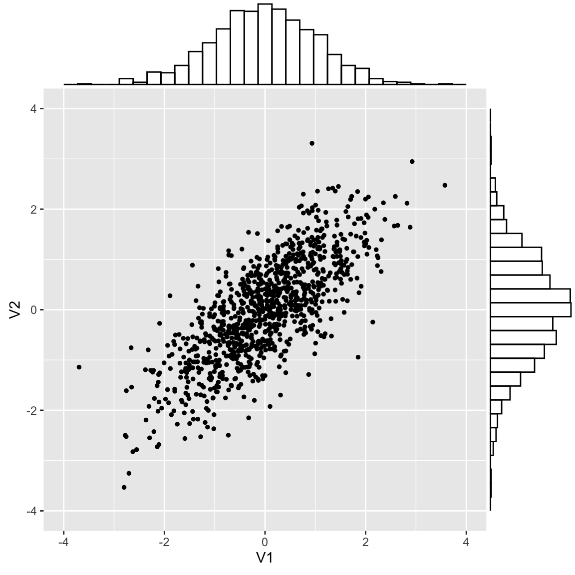
This is called a multinormal distribution
Correlation defines the shape
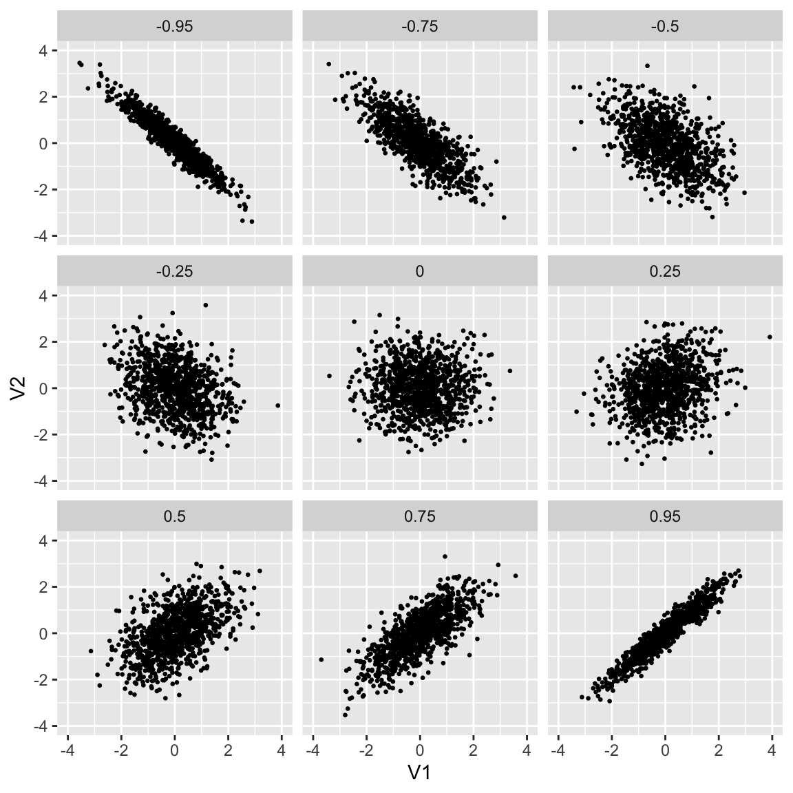
The important part
Ignoring the constants, replacing \(𝐲 = 𝐱-𝐮,\) and taking logarithms, we have that the probability depends on \[𝐲^T Σ^{-1} 𝐲\] so the relationship between the genes is given by \[K=Σ^{-1}\]
This \(K\) is called the precision matrix
(remember that the vector \(𝐲\) components are the gene expressions)
It is not the covariance, but the inverse of the covariance
Example
\[\begin{aligned}
K&=\begin{pmatrix}
1.00 & -0.25 & 0.0\\
-0.25 & 1.00 & 0.3\\
0.00 & 0.30 & 1.0\\
\end{pmatrix}\\
\Sigma&=\begin{pmatrix}
1.0737 & 0.2949 & -0.0884\\
0.2949 & 1.1799 & -0.3539\\
-0.0884 & -0.3539 & 1.1061\\
\end{pmatrix}\end{aligned}
\]
Covariance does not reflect the real relationships
Estimating the precision matrix
As usual, the problem is that we do not know the real covariance, only the sample covariance
Moreover, if we have less samples than genes, then the sample covariance matrix cannot be inverted
Instead, we use methods to calculate pseudo-inverses
We will see one of these methods
Sparse matrices
One condition we can require from our solution is that each gene interacts only with a small number of genes
In general we do not expect that each of the thousand of genes interacts with most of the other thousands of genes
In other words, we expect that the adjacency matrix has mostly zeros
Matrix where the majority of the values are zero are called sparse
Lasso in linear models
Lasso is a method used in linear models to force sparse coefficients
Instead of minimizing \(\sum_i \left(y_i - \sum_j β_j x_{ij}\right)^2,\) the lasso method minimizes \[\sum_i \left(y_i - \sum_j β_j x_{ij}\right)^2 - λ \sum_j\vert \beta_j\vert\]
The parameter \(λ\) has to be chosen by us.
Larger \(λ\) means sparser \(β_j,\) but bigger error
Graphical lasso
Using the same philosophy, one way to find a sparse pseudo-inverse of \(\Sigma\) is to find \(K\) that minimizes \[\log\det(K)-\text{tr}(Σ K) -λ\Vert K\Vert_1\]
Of course, this is done by the computer for us
We only must pay attention to \(λ\)
Graphical lasso gives a family of possible networks
Depending on the value of \(\lambda,\) the result graphical lasso will be more or less sparse
That means that the networks will have more or less edges
