Class 6: Chebyshev Inequality
Methodology of Scientific Research
Andrés Aravena, PhD
28 April 2021
What we know so far
- Experiments are small samples of a large population
- There is variability in the population
- There is noise in every measurement
- We want to understand the population, but we only have a sample
- We want to separate signal and noise
Backwards reasoning
- First, we will assume that we know the population
- We will predict what can happen in any random sample
- We will compare the predicted sample with the experimental one
- Then we will analyze what does this teach us about the population
About the population
We will do an experiment that we call \(X\). Let’s assume that we know
- The set \(Ω\) of all possible outcomes
- The probability \(ℙ(X=x)\) of each outcome \(x∈Ω\)
Then we can calculate
- the expected value \(𝔼X\) a.k.a. population mean
- the population variance \(𝕍X\)
Example
- The experiment is to ask the age of a random person
- Population is “the age of every people living in Turkey”
- \(Ω\) is the natural numbers ≤200
- \(ℙ(X=x)\) is the proportion of people with age \(x\)
- \(𝔼X\) is the average age of people in Turkey
- \(𝕍X\) is the variance of age of people in Turkey
Let’s calculate
Values estimated for 2020
| age range | proportion | males | females |
|---|---|---|---|
| 0-14 | 23.41% | 9,823,553 | 9,378,767 |
| 15-24 | 15.67% | 6,564,263 | 6,286,615 |
| 25-54 | 43.31% | 17,987,103 | 17,536,957 |
| 55-64 | 9.25% | 3,764,878 | 3,822,946 |
| 65+ | 8.35% | 3,070,258 | 3,782,174 |
What are the population mean and variance?
What to expect as outcome
The expected value does not tell us exactly what to expect
But it tells us approximately. We have \[ℙ(𝔼X-c\sqrt{𝕍X} ≤ X ≤ 𝔼X+c\sqrt{𝕍X})≥ 1-1/c^2\] That is, outcomes are probably close to the expected value
\(c\) is a constant that tells us how many standard deviations we need to increase the probability of getting an outcome close to the expected value
This is Chebyshev’s inequality

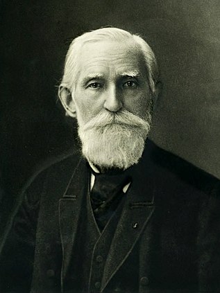
Proved by Pafnuty Lvovich Chebyshev (Пафну́тий Льво́вич Чебышёв) in 1867
It is always valid, for any probability distribution
Later we will see better rules valid only for specific distributions
Alternative formula
Chebyshev inequality can also be written as \[ℙ(|X-𝔼X|≤ c⋅\sqrt{𝕍X})≥ 1-1/c^2\]
The probability that “the distance between the mean \(𝔼X\) and any element \(X\) is less than \(c⋅\sqrt{𝕍X}\)” is greater than \(1-1/c^2\)
Some examples of Chebyshev’s inequality
\[ℙ(𝔼X -c⋅\sqrt{𝕍X}≤ X ≤ 𝔼X +c⋅\sqrt{𝕍X})≥ 1-1/c^2\]
Replacing \(c\) for some specific values, we get
\[\begin{aligned} ℙ(𝔼X-1⋅\sqrt{𝕍X}≤ X ≤ 𝔼X+1⋅\sqrt{𝕍X})&≥ 1-1/1^2=0\\ ℙ(𝔼X-2⋅\sqrt{𝕍X}≤ X ≤ 𝔼X+2⋅\sqrt{𝕍X})&≥ 1-1/2^2=0.75\\ ℙ(𝔼X-3⋅\sqrt{𝕍X}≤ X ≤ 𝔼X+3⋅\sqrt{𝕍X})&≥ 1-1/3^2=0.889 \end{aligned}\]
For any numerical population
- at least 3/4 of the population lie within two standard deviations of the mean, that is, in the interval with endpoints \(𝔼X±2⋅\sqrt{𝕍X}\)
- at least 8/9 of the population lie within three standard deviations of the mean, that is, in the interval with endpoints \(𝔼X±3⋅\sqrt{𝕍X}\)
- at least \(1-1/c^2\) of the population lie within \(c\) standard deviations of the mean, that is, in the interval with endpoints \(𝔼X±c⋅\sqrt{𝕍X},\) where \(c\) is any positive number greater than 1
Exercise
What are the age intervals that contain
- at least 75% of Turkish population
- at least 8/9 of Turkish population
- at least 99% of Turkish population
Proof of Chebyshev Inequality
(read this if you want to know the truth)
A tool that we need
If \(Q\) is a yes-no question, we will use the notation \(〚Q〛\) to represent this:
\[〚Q〛=\begin{cases} 1\quad\text{if }Q\text{ is true}\\ 0\quad\text{if }Q\text{ is false} \end{cases}\]
It is a nice way to write sums limits
Instead of cramming symbols over and under ∑ \[\sum_{x=1}^{10} f(x)\] we can write the limits at normal size \[\sum_x f(x) 〚1≤x≤10〛\]
It is a nice way to decompose events
If we want to calculate the probability of the event \(Q\), instead of writing \[ℙ(Q)=\sum_{x\text{ makes }Q\text{ true}}ℙ(X=x)\] we can write \[ℙ(Q)=\sum_{x}ℙ(X=x) 〚Q(x)〛\]
Proof of Chebyshev’s inequality
By the definition of variance, we have \[𝕍(X)=𝔼(X-𝔼X)^2=\sum_{x∈Ω} (x-𝔼X)^2ℙ(X=x)\] If we multiply the probability by a number that is sometimes 0 and sometimes 1, the right side has to be smaller \[𝕍(X)≥\sum_{x∈Ω} (x-𝔼X)^2ℙ(X=x)〚(x-𝔼X)^2≥α〛\]
We want to make it even smaller
Proof of Chebyshev’s inequality
Since we are only taking the cases where \((X-𝔼X)^2≥α\), replacing \((X-𝔼X)^2\) by \(α\) will make the right side even smaller
\[\begin{aligned} 𝕍(X)& ≥α\sum_{x∈Ω} ℙ(X=x)[(x-𝔼X)^2≥α]\\ & =αℙ\left((X-𝔼X)^2≥α\right) \end{aligned}\] Then we can divide by \(\alpha\) and we get Chebyshev’s result \[ℙ\left((X-𝔼X)^2≥α\right)≤𝕍(X)/α\]
Using the inequality
Chebyshev’s result is \(ℙ\left((X-𝔼X)^2≥α\right)≤𝕍(X)/α.\)
If we choose \(α=c^2⋅𝕍X\) then we have \[ℙ\left((X-𝔼X)^2 ≥ c^2⋅𝕍X \right)≤ 1/c^2\] If we get rid of the squares, we get \[ℙ(|X-𝔼X| ≥ c\sqrt{𝕍X})≤ 1/c^2\] This is the probability that the outcome is far away from the expected value
Probability of being near 𝔼X
Now we can look at the opposite event \[ℙ(|X-𝔼X| ≤ c\sqrt{𝕍X})≥ 1-1/c^2\] The event inside \(ℙ()\) can be rewritten as \[-c\sqrt{𝕍X} ≤ X-𝔼X ≤ c\sqrt{𝕍X}\] which means that the outcome is near the expected value \[𝔼X-c\sqrt{𝕍X} ≤ X ≤ 𝔼X+c\sqrt{𝕍X}\]
Another point of view
The event inside \(ℙ()\) is \(|X-𝔼X| ≤ c\sqrt{𝕍X}\)
As we said, it can be rewritten as \[-c\sqrt{𝕍X} ≤ X-𝔼X ≤ c\sqrt{𝕍X}\] which also means that the expected value is near the outcome \[X-c\sqrt{𝕍X} ≤ 𝔼X ≤ X+c\sqrt{𝕍X}\]
This is a confidence interval