Francis Galton, his cousin and his machine
Francis Galton
![]()
English explorer, Inventor, Anthropologist
(1822–1911)
Francis Galton
He studied medicine and mathematics at Cambridge University.
He invented the phrase “nature versus nurture”
In his will, he donated funds for a professorship in genetics to University College London.
Simulated Galton Machine
![]()
Simulating the Galton Machine
We take each ball independently
In every level, the ball bounces either left or right
We represent these options as -1 and 1
At the last level the position is the sum of all bounces
Simulating the Galton Machine
We will simulate each ball one by one
one_ball <- function(M) {
    bounces <- sample(c(-1, 1), size=M, replace=TRUE)
    return(sum(bounces))
}
Here M is the number of “left-right” choices made by the ball
In other words, M is the number of levels
Simulating the Galton Machine
Galton <- replicate(1000, one_ball(M=5))
barplot(table(Galton))

Larger M, larger variance
Galton <- replicate(10000, one_ball(M=50))
barplot(table(Galton))

Bigger M gives wider results

How Variance Grows

Better use log-log scale

Mean and Variance
It is easy to see that the population mean is 0 for any M
The previous plot shows that the variance is M
Thus, standard deviation will be sqrt(M)
correcting variance for M=5
Galton <- replicate(10000, one_ball(5))/sqrt(5)
barplot(table(Galton))
 Notice that the
 x is not an integer anymore
correcting variance for M=50
Galton <- replicate(10000, one_ball(50))/sqrt(50)
barplot(table(Galton))

correcting variance for M=500
Galton <- replicate(100000, one_ball(500))/sqrt(500)
barplot(table(Galton))

correcting variance for M=5000
Galton <- replicate(100000, one_ball(5000))/sqrt(5000)
barplot(table(Galton))

When M is big, we get Normal distribution

The Normal distribution
This “bell-shaped” curve is found in many experiments, especially when they involve the sum of many small contributions
- Measurement errors
- Height of a population
- Scores on University Admission exams
It is called Gaussian distribution, or also Normal distribution
The Central Limit Theorem
“The sum of several independent random variables converges to a Normal distribution”
The sum should have many terms, they should be independent, and they should have a well defined variance
(In Biology sometimes the variables are not independent, so be careful)
Normal distribution
 Here outcomes are real numbers
Any real number is possible
Probability of any \(x\) is zero (!)
We look for probabilities of intervals
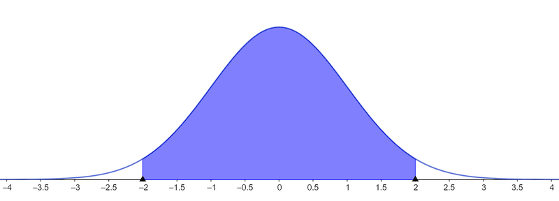
Probabilities of Normal Distribution
![]()
≈95% of normal population is between \(-2\cdot\text{sd}(\mathbf x)\) and \(2\cdot\text{sd}(\mathbf x)\)
≈99% of normal population is between \(-3\cdot\text{sd}(\mathbf x)\) and \(3\cdot\text{sd}(\mathbf x)\)
Simulating the Normal distribution
Instead of simulating the Galton machine several times, we can simulate the Normal distribution using the R function
rnorm(n, mean = 0, sd = 1)
The parameter n is mandatory. It is the sample size
You can also change the mean and the standard deviation of the simulation