Class 18: Complex random systems
Computing for Molecular Biology 2
Andrés Aravena, PhD
7 May 2021
Decomposition again
If the system we want to simulate is complex, we usually do not know the probabilities
In that case we can decompose the random system
- small parts are easier to simulate
- combine them to make the complex system
Let’s experiment with two dice 🎲 🎲
We roll two dice. What is the sum 🎲 +🎲 ?
[1] 9The output is a random outcome
Let’s do 200 experiments
  [1]  5  8  8 10  7  5  8  4  5  6  5  3  9 10  4  9  7  2  5  9  8
 [22]  7  7  9  7  2  4 11  3  8 12  9  7  8  3  9 11  4 10  7  4 10
 [43]  7  9 11  9  7  8  4  6  4 10 10  7 12  9  9  4  7 12  5 11  8
 [64]  8 10  8  7  3  7  7  5 12  5  9  7  9  8  7  5  7  7 10  5 11
 [85]  7  6  9 11 10  3  3 10  3  9  8  5  2 10  5 11  8  4  6  3  9
[106]  2  6 12  9  3  3  3  7  8  9  3 10  8  6  6  7  7  3  6  6  6
[127]  6  7  8  6  6  9 10  6  6  3  3  6  5  7  5  7 11  4 10  7  6
[148]  8  5  4 11  7  6  8  5  9  8 10  4  7  7  5  9  7  8  6  3  7
[169]  4  7 10  9 10  3  3  5  4  6  8 11  9  8  9  3  5  9  6  6  8
[190]  8  6  9  2  7  9  4  6  5  4  8
We can even make a plot
Absolute frequency
- Absolute frequency is how many times we see each value
- The sum of all absolute frequencies is the Number of cases
- Here the number of cases is 200
Increasing the number of cases
All numbers increase
Relative frequency
- Relative frequency is the proportion of each value in the total
- The sum of all relative frequencies is always 1 \[\text{Relative frequency} = \frac{\text{Absolute frequency}}{\text{Number of cases}}\]
Plotting relative frequencies, N=200
Plotting relative frequencies, N=1000
Plotting relative frequencies, N=40000
Empirical Frequencies are close to Probabilities
The result of our experiments give us empirical frequencies
They are close to the theoretical probabilities
When size is bigger, the empirical frequencies are closer and closer to the real probabilities
We know for sure that when size grows we will get the probabilities
But size has to be really big
We are absolutely sure about this
How can be really sure that when size grows we will get the probabilities?
How do we know?
We know because people has proven a Theorem
It is called Law of Large Numbers
Theorems are Eternal Truth
Mathematics is not really about numbers
Mathematics is about theorems
Finding the logical consequences of what we know
But it is all in our mind
Experiments give Nature without Truth
Math gives Truth without Nature
Science gives Truth about Nature
Events
Combining outcomes
We can combine several outcomes in a logic question
An event is any logic question about an outcome
deney == 7deney > 9deneyis even
A way to get absolute frequency
If we want to know how may times we rolled a 7, we can do
[1] 6658Remember that:
- Comparisons produce logic vectors
sum()of a logic vector is the number ofTRUE
Relative frequency
An event is a logic vector.
sum(event) is a number between 0 and length(event)
The relative frequency is
or, better
Exercise: GC content
GC content of DNA fragment
What is the GC content of a random DNA fragment?
You can see that GC content is a random variable
size is the DNA fragment size. Symbol | means or
Simulate GC content
gc_of_fragment <- function(size) {
    dna <- sample(c("A", "C", "G", "T"), size=size, replace=TRUE)
    return(sum(dna=="C" | dna=="G")/size)
}
gc_several <- replicate(10000, gc_of_fragment(900))
hist(gc_several)
Histogram of relative frequencies
Better GC content
We can have a better simulation if we use the real proportions for ("A","C","T","G")
Let’s evaluate them for Carsonella rudii
library(seqinr)
genome <- toupper(read.fasta("AP009180.fna")[[1]])
prob <- c(mean(genome=="A"), mean(genome=="C"),
          mean(genome=="G"), mean(genome=="T"))
prob
[1] 0.41797046 0.08455988 0.08108379 0.41638587Simulate again
gc_of_fragment <- function(size, prob) {
    dna <- sample(c("A", "C", "G", "T"), size=size, prob=prob, replace=TRUE)
    return(sum(dna=="C" | dna=="G")/size)
}
gc_several <- replicate(10000, gc_of_fragment(900, prob))
hist(gc_several, probability=TRUE)
Range of GC content depends on fragment size
small_fragments <- replicate(10000, gc_of_fragment(200, prob))
medium_fragments <- replicate(10000, gc_of_fragment(600, prob))
big_fragments <- replicate(10000, gc_of_fragment(1200, prob))
Another view of GC content v/s size
Other random variables?
What other Random Variables can you imagine?
- Average
- Number of trials until success
- Number plants that grow in the lab
- Number of people that answer the homework
- Number of people that passes the course
What other random variable do you see?
How many times will you do this course?
Depending on how many questions you ask and how many homework you do, you will have different chances of passing this course
To be neutral, let’s try with different probabilities
How many times do you need to do this course until you pass?
Counting until success
Assuming we have a function called fail(), that returns TRUE when the experiment fails; then this code gives us number of trials until success
Success & Failure: two sides of a coin
A simple way to model fail() is to use a coin
or, better
A biased coin
This function takes one input: the probability of success
Tossing a coin until Heads
Results for 50%
Results for 90%
Results for 10%
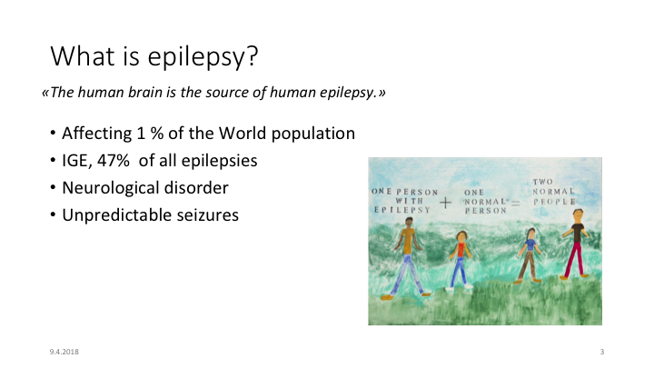
Epilepsy


How many persons with epilepsy in our course?
Worldwide proportion is 1%
And world is a population
We are 99 people in this course, including me
Can we have 5 people with epilepsy in our class?
Do we have the same Birthday?
Same Birthday
What are the chances that two people have the same birthday in our class?