Class 6: Local DNA statistics
Computing for Molecular Biology 2
Andrés Aravena, PhD
26 March 2021
Why we do statistics on the sequence?
Statistics tells a story that makes sense of the data
In genomics, we look for biological sense
That story can be global: about the complete genome
Or can be local: about some region of the genome
Last class we saw global properties
Local statistics
Local statistics look only through a small window
A window is a part of the genome,
- from an initial position,
- and with a fixed size
For example, we can analyze a region of 500 bp starting at position 3000 of the genome
First, we load E.coli genome
library(seqinr)
chromosomes <- read.fasta("NC_000913.fna", seqtype="DNA", set.attributes = FALSE)
length(chromosomes)
[1] 1
genome <- chromosomes[[1]]
length(genome)
[1] 4641652
Remember the GC content function
This is version 3, but we use a shorter name
gene_GC_content <- function(dna) {
    V <- toupper(dna)
    count_C <- sum(V=="C")
    count_G <- sum(V=="G")
    GC_content <- (count_C +count_G)/length(V)
    return(GC_content)
}
This is a global statistic. Test it with the complete genome
[1] 0.5079071
Application
Calculate the GC content for only part of the genome
Instead of all the genome, we only look through a window
The result should depend on:
- the position of the window
- the size of the window
- the genomic sequence
In plain English
- Inputs are
position, size, and dna
- we know how to calculate GC content of a complete sequence
- we can use
gene_GC_content()
- we need to “cut”
dna in a fragment starting at position
- the fragment must be of length
size
- we need to use indices starting at
position
- the vector of indices must be of length
size
Write the function
The new function looks like this
window_GC_content <- function(position, size, dna) {
    # we need to use indices starting at `position`
    # the vector of indices must be of length `size`
    # we need to "cut" `dna` using the indices
    # we use `gene_GC_content()` on the dna fragment
    return(answer)
}
What should be the code?
Remember the seq() function
seq(from, to, by, length.out)
All inputs are optional
Choose carefully which ones to use
Examples of seq()
[1] 5 6 7 8 9 10 11 12 13 14
seq(from=5, length.out=10)
[1] 5 6 7 8 9 10 11 12 13 14
[1] 5 8 11 14 17 20 23 26 29
Looking at the window
position 3000, size 500
window <- genome[seq(from=3000, length.out=500)]
In the general case, we can write
window <- genome[seq(from=start, length.out=size)]
Our code
window_GC_content <- function(position, size, dna) {
    # we need to use indices starting at `position`
    # the vector of indices must be of length `size`
    indices <- seq(from=position, length.out=size)

    # we need to "cut" `dna` using the indices
    window <- dna[indices]

    # we use `gene_GC_content()` on the dna fragment
    answer <- gene_GC_content(window)
    return(answer)
}
Using our code in many places
We traverse the genome with several windows of fixed size
Each window starts after the end of the previous one
In other words, the windows do not overlap
![]()
Create a vector with the window’s positions
We start at the first DNA position, until the last
Be careful to not step out of DNA
win_pos <- seq(from=1, to=length(genome)-size, by=size)
Now we apply window_GC_content to each element of win_pos
sapply(win_pos, window_GC_content, window_size, genome)
The result depends on window_size
Results
win_pos <- seq(from=1, to=length(genome)-1E4, by=1E4)
gc <- sapply(win_pos, window_GC_content, 1E4, genome)
plot(gc)

We can also use pipes
library(magrittr)
seq(from=1, to=length(genome)-1E4, by=1E4) %>%
    sapply(window_GC_content, 1E4, genome) %>% plot()

GC Skew through the genome
GC Skew
What is the ratio of \(G-C\) respect to \(G+C\)?
Calculate the ratio \[\frac{G-C}{G+C}\]
using several windows. What do you see?
We use the function from last class
calculate_GC_skew <- function(dna) {
    V <- toupper(dna)
    count_C <- sum(V=="C")
    count_G <- sum(V=="G")
    GC_skew <- (count_G-count_C)/(count_C+count_G)
    return(GC_skew)
}
Test it with the complete genome
calculate_GC_skew(genome)
[1] -0.001125755
Same logic for the “windowed” version
window_GC_skew <- function(position, size, dna) {
    # we need to use indices starting at `position`
    # the vector of indices must be of length `size`
    indices <- seq(from=position, length.out=size)

    # we need to "cut" `dna` using the indices
    window <- dna[indices]

    # we use `calculate_GC_skew()` on the dna fragment
    answer <- calculate_GC_skew(window)
    return(answer)
}
Evaluate gc_skew() window by window
win_pos <- seq(from=1, to=length(genome)-1E4, by=1E4)
gc <- sapply(win_pos, window_GC_skew, 1E4, genome)
plot(gc, type="l", xlab="Position in the Genome", ylab="GC skew")
abline(h=0,col="red")

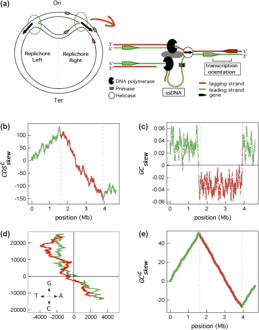
GC skew and genome replication
GC skew changes sign at the boundaries of the two replichores
This corresponds to DNA replication origin or terminus
The replication origin is usually called ori.
DNA replication
![]()
Marie Touchon, Eduardo P.C. Rocha, (2008), From GC skews to wavelets: A gentle guide to the analysis of compositional asymmetries in genomic data,
Biochimie, Volume 90, Issue 4,