Class 19: Overlay-Layout-Consensus Assembly & Statistics
Bioinformatics
Andrés Aravena
16 December 2021
There are basically three strategies used to assemble genomes
Greedy algorithms
Overlap – Layout – Consensus
De Bruijn graphs
Today we will speak about the first two strategies
Greedy algorithm
Given a set of sequence fragments, the object is to find a longer sequence that contains all the fragments.
- Evaluate the pairwise alignments of all fragments
- Choose two fragments with the largest overlap
- Merge the chosen fragments
- Repeat step 2 and 3 until only one fragment is left.
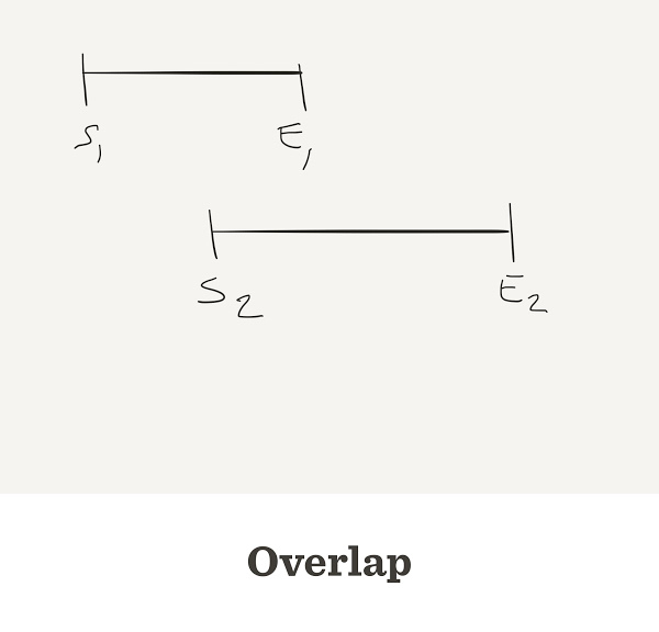
Overlap
- All reads are compared to each other
- and to their reverse-complement
- The alignment considers each base’s quality
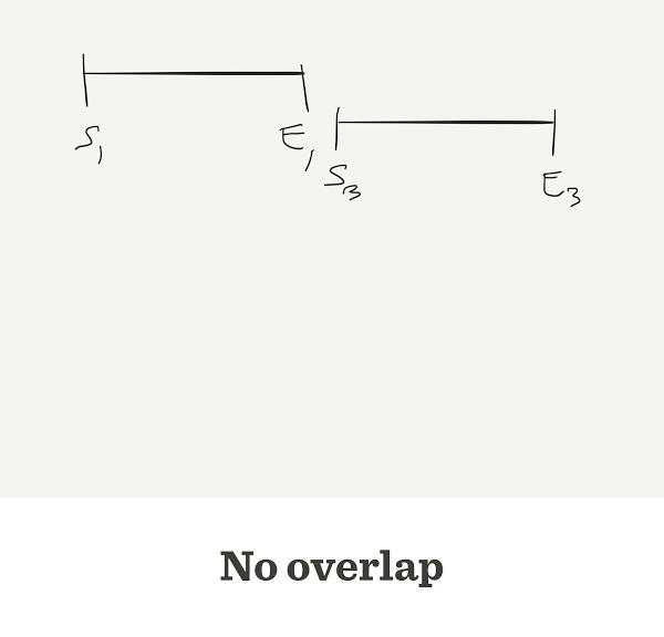
- When the end of one read matches the start of another read, we say that they overlap
Sometimes reads do overlap
Sometimes they do not overlap
Problems with the greedy approach
The final sequence may be wrong
Two different reads A, B may match the same read X
To decide which one is correct, a Layout stage is used
Layout
In this approach, the overlap between reads is used to build a graph of reads relationships
This graph determines the layout of all reads,
that is, their relative positions
Contigs
Usually there are several independent groups of reads that are not connected in the layout graph
(we say that the graph has several connected components)
All the reads that are connected together form a contig
Consensus
Once the layout is clear, the last step is to retrieve the consensus sequence of the contig
In fact, it is not a consensus. It is a vote. The majority wins
High quality votes are more important than low quality ones
Example: Phrap assembler
The human genome project used Phred for base-calling and Phrap for assembly
Phrap produces several files. The most important has extension .ace
These programs are free for academic usage (non-commercial)
Example ACE file
AS 36 39

CO Contig1| 131 1 1 U
gctagaaaaaaaaggactcccagtagaaatacgtacaataaagtaggttc
ctctagttaactgttacaaaataagtttcccattggtaatataatagatt
tataactgttatatccagagcaacctagggg

BQ
15 15 15 15 15 15 15 15 15 15 15 15 15 15 15 15 15 15 15 15 15 15 15 15 15 15 15
15 15 15 15 15 15 15 15 15 15 15 15 15 15 15 15 15 15 15 15 15 15 15 15 15 15 15
15 15 15 15 15 15 15 15 15 15 15 15 15 15 15 15 15 15 15 15 15 15 15 15 15 15 15
15 15 15 15 15 15 15 15 15 15 15 15 15 15 15 15 15 15 15 15 15 15 15 15 15 15 15
15 15 15 15 15 15 15 15 15 15 15 15 15 15 15 15 15 15 15 15 15 15 15

AF 5765593 U 1
BS 1 131 5765593

RD 5765593 131 0 6
gctagaaaaaaaaggactcccagtagaaatacgtacaataaagtaggttc
ctctagttaactgttacaaaataagtttcccattggtaatataatagatt
tataactgttatatccagagcaacctagggg
Example ACE file (last part)
CO Contig36 111 2 63 U
taTAAAGTCGATGGGGAGGAAGATAGGGGAGCTAAAGCCATAGGGAAACC
ACGTAGTTCTGCGTCAAGCGTTgccttcCGAGGTGCTCTCCGCTTTTCCA
TGCtccaatcg

BQ
15 15 25 25 25 25 25 25 25 25 25 25 25 25 25 25 25 25 25 25 25 25 25 25 25 25 25
25 25 25 25 25 25 25 25 25 25 25 25 25 25 25 25 25 25 25 25 25 25 25 25 25 25 25
25 25 25 25 25 25 25 25 25 25 25 25 25 25 25 25 25 25 15 15 15 15 15 15 25 25 25
25 25 25 25 25 25 25 25 25 25 25 25 25 25 25 25 25 25 25 25 25 25 15 15 15 15 15
15 15 15

AF 5648323 U 1
AF 5703145 U 1
Assembly statistics
Assembly Statistics
When we report an assembly result, we describe
- Number of contigs
- Depth of coverage
- Breadth of coverage
- N50
Assembly input parameters
The assembly result depends on
- Length of the Genome: \(G\)
- Length of reads: \(L\)
- Number of reads: \(N\)
In general \(L\) can be different for each read
For this class we will assume all reads have the same length
The genome length \(G\) is usually an estimation, based on wet-lab experiments (flow cytometry)
Depth

Depth is a property of each genome position
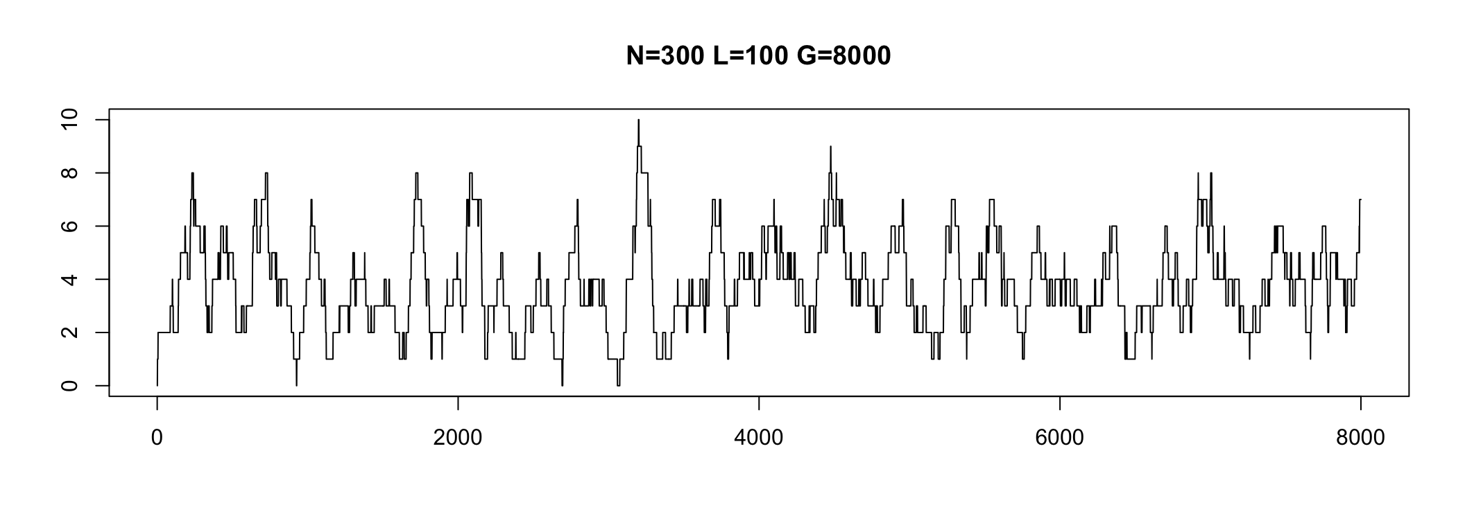
In practice, some genome parts have coverage 0
We do not see these regions
Depth varies in a range
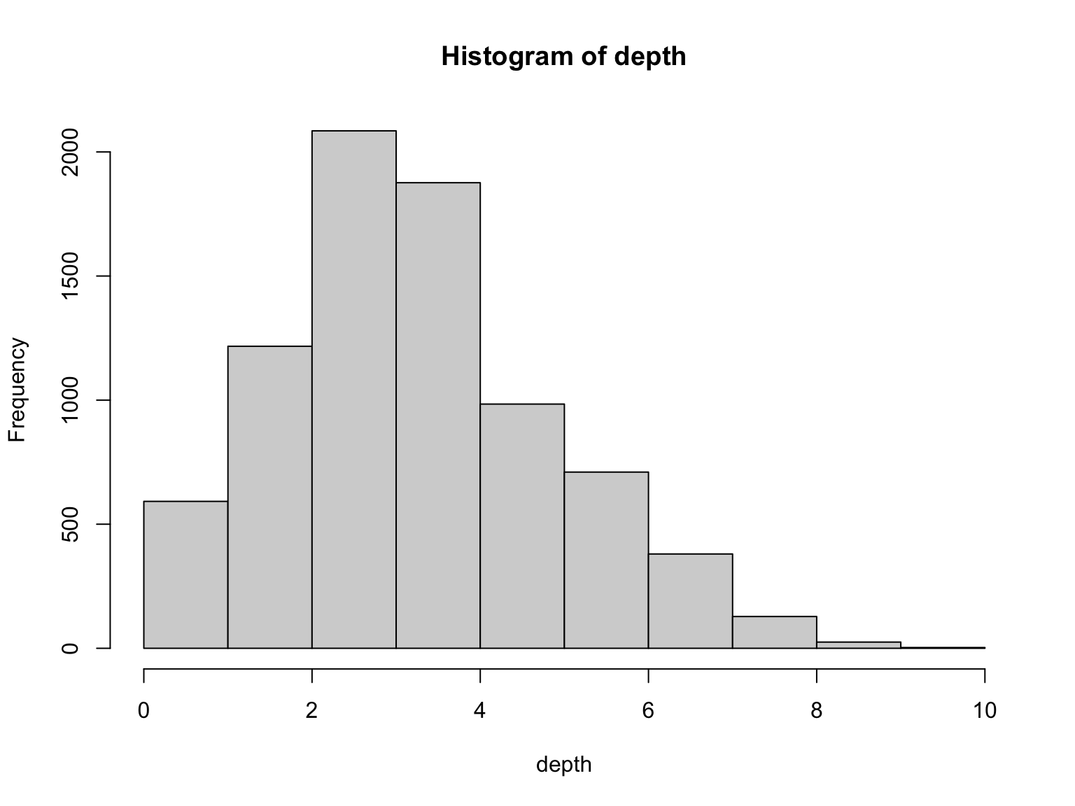
Average Depth
The average number of times that a particular nucleotide is represented in a collection of reads
Average Depth is sometimes called Coverage
Depth average is also known as coverage
Coverage can be calculated before sequencing \[ \text{Coverage} = \frac{NL}{G} \]
Breadth of Coverage
Percentage of bases that are sequenced a given number of times
- Example
- genome sequencing 30× average depth can achieve a 95% breadth of coverage of the reference genome at a minimum depth of ten reads
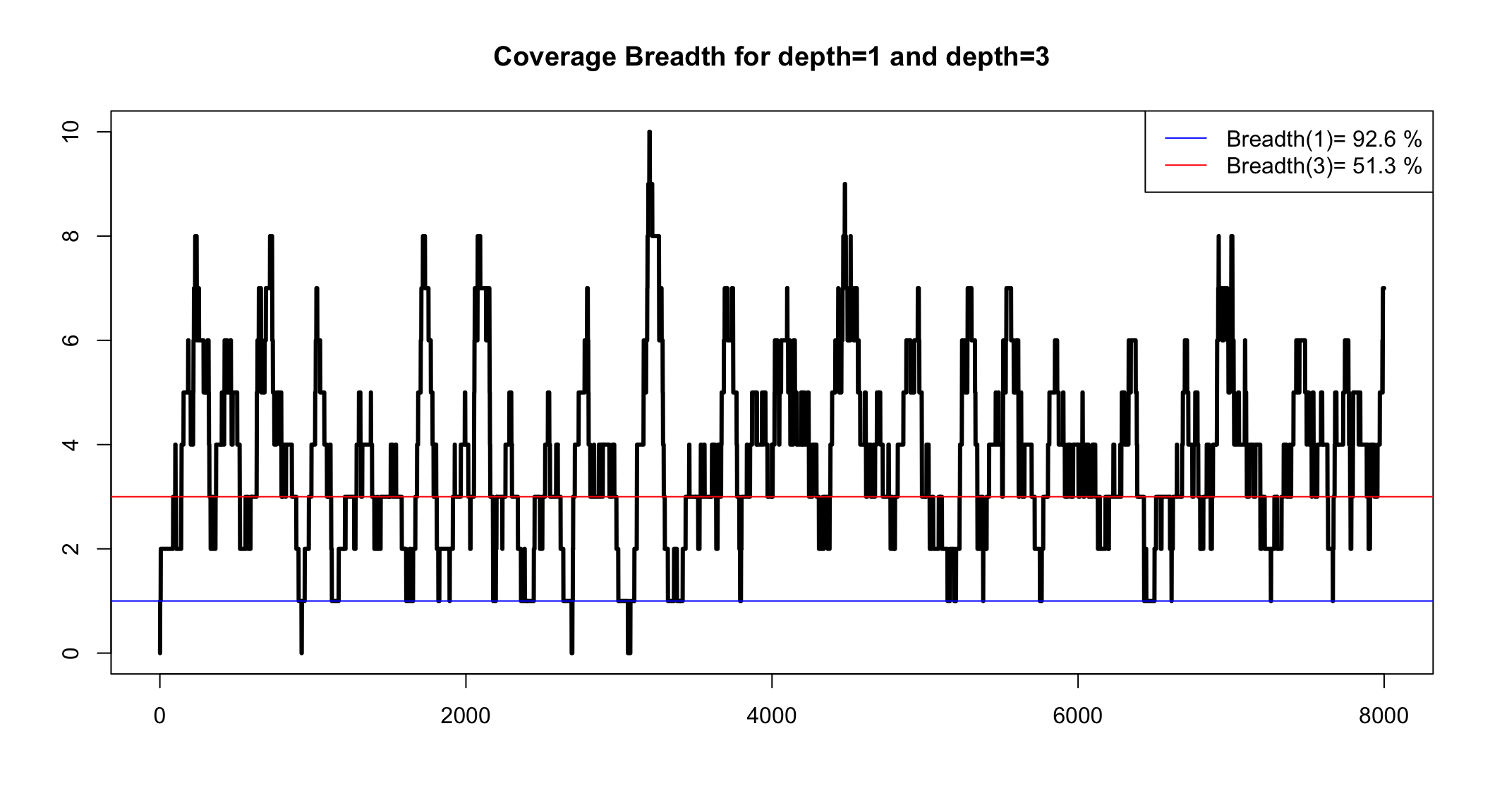
Coverage Breadth
This is the percentage of the genome that we can see with our reads
More precisely, it is the percentage of the genome that has coverage over a minimum
We can only know coverage breadth after we assembly
Coverage breadth for a minimum depth
We can simulate to see the range
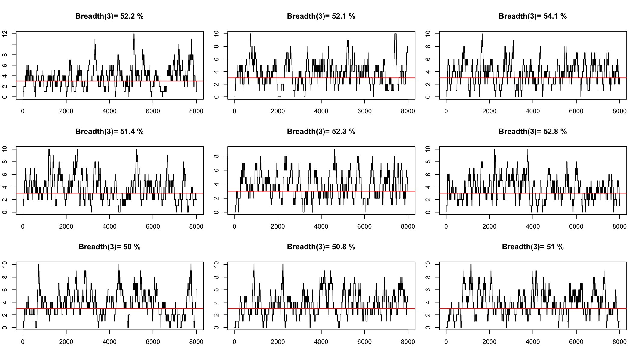
Simulate to get a confidence interval
The question we want to answer is
How many reads we need to see all the genome with a minimum depth?
How would you answer that question?