Class 25: Polynomial Models
Computing for Molecular Biology 1
Andrés Aravena, PhD
4 January 2021
Modeling free fall
##
## Attaching package: 'dplyr'
## The following objects are masked from 'package:stats':
##
## filter, lag## The following objects are masked from 'package:base':
##
## intersect, setdiff, setequal, unionExample videos
YouTube has an option to show the video at 0.25 speed. Try it
- In your computer, open a new text file and write the experimental data
- three columns: msec, position, and replica
- one row for each time the object crosses a mark
Summary of the video
Replicas
Every serious experiment should be repeated at least 3 times
Without replication, it can be wrong
Replicas indicate that the result is repetible
Technical and biological replicas
In molecular biology we have two kinds of replicas
- Technical replicas
- the same organism, measured several times
- Biological replicas
- different organisms, measured at least one time
Technical and biological replicas
Technical replicas give you precise measurements of a single individual
This is what we do in Medicine
Biological replicas gives you data about one or more species
That is what we do in Science
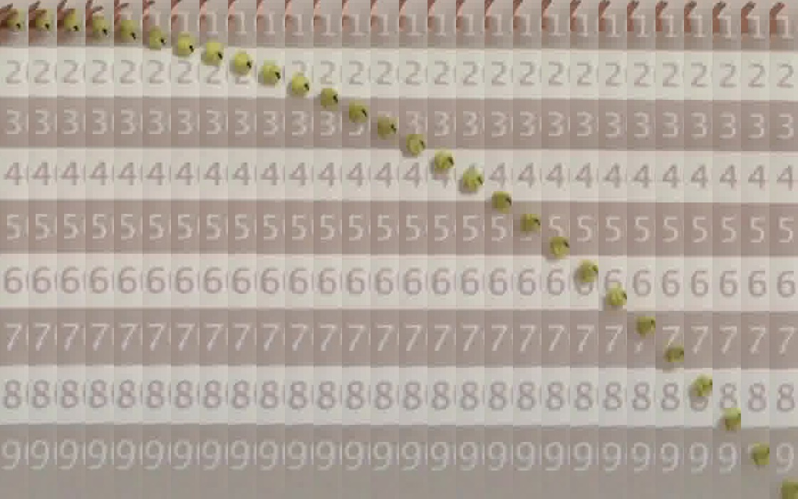
“Free fall” experiment
An ideal falling ball

Simulated data
| height | speed | time |
|---|---|---|
| 2.0000 | -0.20 | 0.0006 |
| 1.9778 | -0.69 | 0.0493 |
| 1.9310 | -1.18 | 0.1009 |
| 1.8598 | -1.67 | 0.1485 |
| 1.7640 | -2.16 | 0.2004 |
| 1.6438 | -2.65 | 0.2511 |
| 1.4990 | -3.14 | 0.2985 |
| 1.3297 | -3.63 | 0.3509 |
| 1.1360 | -4.12 | 0.4018 |
| 0.9177 | -4.61 | 0.4515 |
| 0.6750 | -5.10 | 0.4997 |
What is the good formula this time?
We can use a logarithmic scale to see if we get a straight line
- If we get straight line in semi-log then the formula is \[y=A\cdot B^x\]
- If we get straight line in log-log then the formula is \[y=A\cdot x^B\]
Semi-Logarithmic scale

Logarithmic scale

This is not any exponential
There are many possible functions that connect \(x\) and \(y\)
We will try a polynomial formula
A polynomial is a formula like \[y=A + B\cdot x + C\cdot x^2 +\cdots+ D\cdot x^n\]
The highest exponent is the degree of the polynomial
We will try a 2-degree formula \[\text{height}=A+B\cdot\text{time}+C\cdot\text{time}^2\]
We really have to add a new column
You may be tempted to use
But that does not work.
Exponents and multiplications in formulas have a different meaning
(that we will see later)
A new column for polynomial model
We need to add an extra column, with the square of the time
  height speed     time   time_sq
1  2.000 -0.20 0.000638 4.070e-07
2  1.978 -0.69 0.049256 2.426e-03
3  1.931 -1.18 0.100938 1.019e-02
4  1.860 -1.67 0.148492 2.205e-02
5  1.764 -2.16 0.200394 4.016e-02
6  1.644 -2.65 0.251069 6.304e-02
Linear model for polynomial
Now we use two independent variables in the model. This is different from the plot() function
Call:
lm(formula = height ~ time + time_sq, data = ball)

Coefficients:
(Intercept)         time      time_sq
      2.000       -0.205       -4.873
Interpretation
We used the formula \[\text{height}=A+B\cdot\text{time}+C\cdot\text{time}^2\] The linear model gave us \[\begin{aligned} A & =2\\ B & =-0.205\\ C & =-4.9 \end{aligned}\]
Predicted v/s original

It works!
Interpretation
What is the meaning of the coefficients? \[\begin{aligned} \text{height} & =A+B\cdot\text{time}+C\cdot\text{time}^2 \\ A & =2\\ B & =-0.205\\ C & =-4.9 \end{aligned}\]
Our experiment
The data
# A tibble: 18 x 3
    msec position replica
   <dbl>    <dbl> <chr>
 1  2355       10 A
 2  2457       20 A
 3  2533       30 A
 4  2558       40 A
 5  2639       50 A
 6  2690       60 A
 7  2742       70 A
 8  2742       80 A
 9  2797       90 A
10  1837       10 B
11  1970       20 B
12  2022       30 B
13  2104       40 B
14  2129       50 B
15  2210       60 B
16  2237       70 B
17  2262       80 B
18  2313       90 B
First view

Let’s keep only replica A
For this class, we will use only the first replica
# A tibble: 9 x 3
   msec position replica
  <dbl>    <dbl> <chr>
1  2355       10 A
2  2457       20 A
3  2533       30 A
4  2558       40 A
5  2639       50 A
6  2690       60 A
7  2742       70 A
8  2742       80 A
9  2797       90 A
Time should start at zero
- We started the timer before dropping the ball
- The first data is when the ball crosses 10
- We can choose this as our time reference
- The ball is already moving
- Initial speed is not zero
- The column name is
msec. It means milliseconds
Normalizing time data
Let’s add a new column, called time, with the correct value of seconds
# A tibble: 9 x 4
   msec position replica  time
  <dbl>    <dbl> <chr>   <dbl>
1  2355       10 A        2.36
2  2457       20 A        2.46
3  2533       30 A        2.53
4  2558       40 A        2.56
5  2639       50 A        2.64
6  2690       60 A        2.69
7  2742       70 A        2.74
8  2742       80 A        2.74
9  2797       90 A        2.80
Normalizing time data
Now we change time to start at 0
# A tibble: 9 x 4
   msec position replica  time
  <dbl>    <dbl> <chr>   <dbl>
1  2355       10 A       0
2  2457       20 A       0.102
3  2533       30 A       0.178
4  2558       40 A       0.203
5  2639       50 A       0.284
6  2690       60 A       0.335
7  2742       70 A       0.387
8  2742       80 A       0.387
9  2797       90 A       0.442
Normalizing position data
We should also transform position to meters. The first data should be at 0
Each black/white strip was a little more than 19 centimeters
# A tibble: 9 x 5
   msec position replica  time height
  <dbl>    <dbl> <chr>   <dbl>  <dbl>
1  2355       10 A       0      0
2  2457       20 A       0.102  0.192
3  2533       30 A       0.178  0.384
4  2558       40 A       0.203  0.576
5  2639       50 A       0.284  0.768
6  2690       60 A       0.335  0.96
7  2742       70 A       0.387  1.15
8  2742       80 A       0.387  1.34
9  2797       90 A       0.442  1.54
Normalized data

We will use a polinomial model
This is a parabola, which can be modeled with a second degree polynomial \[y=A + B\cdot x + C\cdot x^2\] When we use a polynomial model, we need to add new columns to our data frame
This is used only for the model
Fitting the model
Call:
lm(formula = height ~ time + time_sq, data = fall)

Coefficients:
(Intercept)         time      time_sq
    0.00131      1.55751      4.26664
(Intercept) should be 0
Since we choose that at time=0 we have height=0, we know that (Intercept) is 0
In other words, our model here is \[y= B\cdot x + C\cdot x^2\] The old \(A\) has a fixed value of 0
How do we do that in R?
Fixing the intercept to 0
Call:
lm(formula = height ~ time + time_sq + 0, data = fall)

Coefficients:
   time  time_sq
   1.57     4.25
Meaning of the coefficients
If you remember your physics lessons, you can recognize that in the formula \[y= B\cdot x + C\cdot x^2\] the value \(B\) is the initial speed, and \(C=-g/2\)
Thus, we can find the gravitational acceleration in the second coefficient