Class 24: Logarithmic models
Computing in Molecular Biology and Genetics 1
Andrés Aravena, PhD
4 January 2021
What is a logarithm?
We need very little math: arithmetic, algebra, and logarithms
Just remember that if \(x=p^m\) then \[\log_p(x) = m\] For example \[\log_{10}(10000) = 4\]
We can change the base
If we use another base, for example \(q\), then \[\log_q(x) = m\cdot\log_q(p)\] For example \[\log_2(10000) = 4\cdot\log_2(10) = 4\cdot 3.3219 = 13.2877\]
We can choose the best base
So if we use different bases, there is only a scale factor
The “easiest” one is natural logarithm
If \(x=\exp(m)\) then \(\log(x)=m\)
In R, log(x) is \(\ln(x)\)
[1] 9.21Other things about logarithms
They only work with positive numbers. Not with 0
If \(x=\exp(m)\) then \[\log(x)=m\]
The important part
If \(x=p\cdot q\) then \[\log(x)=\log(p)+\log(q)\]
If \(x=a^m\) then \[\log(x)=m\log(a)\]
Linear models can be used in three cases
Basic linear model \[y=A+B\cdot x\] Exponential change (Initial value and growth Rate) \[y=I\cdot R^x\] Power law (Constant and Exponent) \[y=C\cdot x^E\]
Linear models can be used in three cases
Basic linear model \[y=A+B\cdot x\] Exponential: if \(y=I\cdot R^x\) then \[\log(y)=\log(I)+\log(R)\cdot x\] Power of \(x\): if \(y=C\cdot x^E\) then \[\log(y)=\log(C)+E\cdot\log(x)\]
Which one to use?
The easiest way to decide is to
- draw several plots, placing
log()in different places, - see which one seems more like a straight line
For example, let’s analyze data from Kleiber’s Law
The following data shows a summary
The complete table has 26 animals
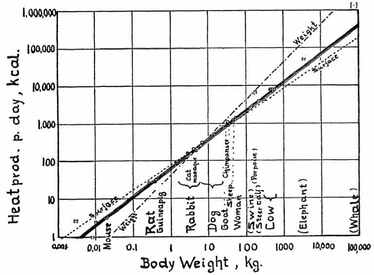
Kleiber’s Law
Body size v/s metabolic rate
| animal | kg | kcal |
|---|---|---|
| Mouse | 0.021 | 3.6 |
| Rat | 0.282 | 28.1 |
| Guinea pig | 0.410 | 35.1 |
| Rabbit | 2.980 | 167.0 |
| Cat | 3.000 | 152.0 |
| Macaque | 4.200 | 207.0 |
| Dog | 6.600 | 288.0 |
| animal | kg | kcal |
|---|---|---|
| Goat | 36.0 | 800 |
| Chimpanzee | 38.0 | 1090 |
| Sheep ♂ | 46.4 | 1254 |
| Sheep ♀ | 46.8 | 1330 |
| Woman | 57.2 | 1368 |
| Cow | 300.0 | 4221 |
| Young cow | 482.0 | 7754 |
First plot: Linear

Second plot: semi-log

Third plot: log-log

Which one seems more “straight”?
The plot that seems more straight line is the log-log plot
Therefore we need a log-log model.
(Intercept)     log(kg)
     4.2058      0.7559
What is the interpretation of these coefficients?
If \(\log(kcal)=4.21 + 0.756\cdot \log(kg)\) then \[kcal=\exp(4.21) \cdot kg^{0.756} =67.1 \cdot kg^{0.756}\]
Therefore:
- For a 1kg animal, the average energy consumption is \(\exp(4.21) = 67.1\) kcal
- The energy consumption increases at a rate of \(0.756\) kcal/kg.
This is Kleiber’s Law
“An animal’s metabolic rate scales to the ¾ power of the animal’s mass”.
Google it
Using the model to predict
What can we do with the model?
Models are the essence of scientific research
They provide us with two important things
An explanation for the observed patterns of nature
A method to predict what will happen in the future
Predicting with the model
where newdata is a data frame with column names corresponding to the independent variables
If we omit newdata, the prediction uses the original data as newdata
Results: What is wrong here?
| animal | kg | kcal | predicted |
|---|---|---|---|
| Mouse | 0.021 | 3.6 | 1.285 |
| Rat | 0.282 | 28.1 | 3.249 |
| Guinea pig | 0.410 | 35.1 | 3.532 |
| Rabbit | 2.980 | 167.0 | 5.031 |
| Cat | 3.000 | 152.0 | 5.036 |
| Macaque | 4.200 | 207.0 | 5.291 |
| Dog | 6.600 | 288.0 | 5.632 |
| animal | kg | kcal | predicted |
|---|---|---|---|
| Goat | 36.0 | 800 | 6.915 |
| Chimpanzee | 38.0 | 1090 | 6.955 |
| Sheep ♂ | 46.4 | 1254 | 7.106 |
| Sheep ♀ | 46.8 | 1330 | 7.113 |
| Woman | 57.2 | 1368 | 7.265 |
| Cow | 300.0 | 4221 | 8.517 |
| Young cow | 482.0 | 7754 | 8.876 |
Undoing the logarithm
We want to predict the metabolic rate, depending on the weight
The independent variable is \(kg\), the dependent variable is \(kcal\)
But our model uses only \(\log(kg)\) and \(\log(kcal)\)
So we have to undo the logarithm, using \(\exp()\)
Correct formula for prediction
| animal | kg | kcal | predicted |
|---|---|---|---|
| Mouse | 0.021 | 3.6 | 3.616 |
| Rat | 0.282 | 28.1 | 25.762 |
| Guinea pig | 0.410 | 35.1 | 34.185 |
| Rabbit | 2.980 | 167.0 | 153.113 |
| Cat | 3.000 | 152.0 | 153.889 |
| Macaque | 4.200 | 207.0 | 198.458 |
| Dog | 6.600 | 288.0 | 279.287 |
| animal | kg | kcal | predicted |
|---|---|---|---|
| Goat | 36.0 | 800 | 1007 |
| Chimpanzee | 38.0 | 1090 | 1049 |
| Sheep ♂ | 46.4 | 1254 | 1220 |
| Sheep ♀ | 46.8 | 1330 | 1228 |
| Woman | 57.2 | 1368 | 1429 |
| Cow | 300.0 | 4221 | 5001 |
| Young cow | 482.0 | 7754 | 7157 |
Visually (log scale)

Visually (linear scale)

In the paper
Moore’s Law
“The robots are coming”
Moore’s Law
![]()
Real data: Number of transistors v/s year

Semilog scale: Number of transistors v/s year

Semi-log means exponential growth
we have straight line on the semi-log
That is, log(y) versus x \[\log(y)=\log(I) + \log(R)\cdot x\] In this case the original relation is \[y=I\cdot R^x\]
Model
(Intercept)        Date
  -677.2050      0.3471
\[ \log(count) = -677.205 + 0.3471\cdot Date \]
Graphically

Undoing logarithms
(Intercept)        Date
 7.828e-295   1.415e+00
\[ count = 7.8275\times 10^{-295} \cdot 1.415^ {Date} \]
Every year “processor power” grows by a factor 1.415
(How many years to get 200% increase?)
In year 0, the processors had \(7.8275\times 10^{-295}\) transistors
Graphically

Meaning
Every year “processor power” grows by a factor of
 Date
1.415
That is, it increases by
Date
41.5
percent
Exercise
Genomic databases
Every time a researcher publishes a paper about DNA sequencing, all the sequences are uploaded to online databases.
One of these databases is https://www.ncbi.nlm.nih.gov/sra/
It contains all DNA reads made with New Generation Sequencers
We want to understand how fast this database is growing
Steps
- Download the file
sra_bases.txt - Create a new Rmarkdown document. Delete all unnecessary text
- do not forget to write your student number
- write the code to read the file into your document
- write the code to produce a plot like the one at https://www.ncbi.nlm.nih.gov/sra/docs/sragrowth/
The plot must look like this
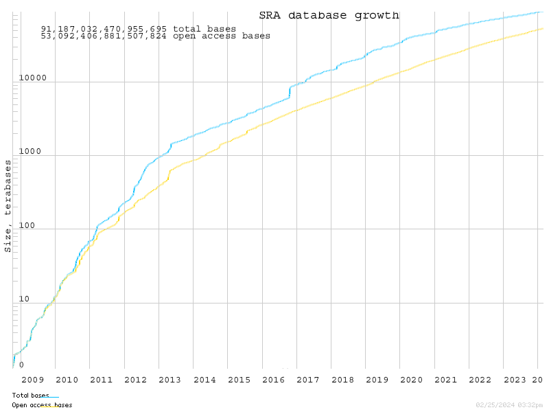
Database growth
- The growth of databases is usually modeled as a semi-log linear model.
- Build a semi-log model and find
- what is the factor of growth per day?
- What will be the database size two years after the last entry in your table?
- write your code and comments in the same Rmarkdown file
Plots: bad ideas
plot(sra):- plots all the data frame
plot(day~log(bases), data = sra):- sideways
plot(log(bases)~log(day), data=sra):- log-log, not semi-log
Good plot
plot(log(bases) ~ day, data = sra)- Good for analysis
Meaning
Call:
lm(formula = log(bases) ~ day, data = sra)

Coefficients:
(Intercept)          day
   28.34146      0.00248
Coefficients are log(bases)
In a semi-log model, we have \[\log(\text{bases}) = \underbrace{\log(\text{initial})}_{\texttt{coef(model)[1]}} + \underbrace{\log(\text{rate})}_{\texttt{coef(model)[2]}} \cdot \text{days}\]
Undoing log(), we have \[\text{bases} = \text{initial}\cdot\text{rate}^\text{days}\]
Thus, \(\text{rate}=\)exp(coef(model)[2])\(=1.0025\)
Meaning of rate
If \(\text{rate}=1.0025\) it means that the database grows \(0.25\%\) every day
- That is \(147.5\%\) every year
- That is \(295\%\) in two years
Predicting the future
To make predictions using the model, we use
We need a data frame with one column named day,
because we used day in the formula
Predicting the next 2 years
The last day in sra is max(sra$day)
Two years after the last will be
so we will use