# A tibble: 117 x 10
   answer_date id    english_level sex   birthdate  birthplace height_cm
   <date>      <chr> <chr>         <fct> <date>     <chr>          <dbl>
 1 2018-09-17  3e50… I can speak … Male  1993-02-01 -/Turkey         179
 2 2018-09-17  479d… I can unders… Fema… 1998-05-21 Kahramanm…       168
 3 2018-09-17  39df… I can read a… Fema… 1998-01-18 Batman/Tu…        NA
 4 2018-09-17  d2b0… I can read a… Male  1998-08-29 Antalya/T…       170
 5 2018-09-17  f22b… I can read a… Fema… 1998-05-03 Izmir/Tur…       162
 6 2018-09-17  849c… İngilizce bi… Fema… 1995-10-09 Yalova/Tu…       167
 7 2018-09-17  8381… I can speak … Fema… 1997-09-19 Adıyaman/…       174
 8 2018-09-17  b0dd… I can read a… Male  1997-11-27 Bursa/Tur…       180
 9 2018-09-17  2972… I can read a… Fema… 1999-01-02 Istanbul/…       162
10 2018-09-17  72c0… I can read a… Fema… 1998-10-02 Istanbul/…       172
# … with 107 more rows, and 3 more variables: weight_kg <dbl>,
#   handedness <fct>, hand_span <dbl>
Plotting a formula
plot(weight_kg ~height_cm, data = students)
Reminder of plot() function
plot(y ~ x) looks like plot(x, y)
Formulas are nice:
plot(y~x, data=dframe)
In general the defaults are good
axis labels are the plotted variable’s names
ranges are automatic
You can choose the horizontal and vertical ranges
Linear models
In science we work by creating models of how nature works
There are several kinds of models
One of the easiest and more commonly used are the linear models
We approximate all our data by a straight line that shows the relationship between some variables, with a formula like \[y=a + b\cdot x\]
A simple model
We want to describe the relationship between weight and height
A basic rule of thumb is that weight in kg is usually equal to height in cm minus 100 \[weight = height - 100\]
That is, the weight is the number of centimeters over one meter
Adding a straight line to a plot
plot(weight_kg ~height_cm, data = students)abline(a =-100, b =1)
A-B-line
This command adds a straight line in a specific position
abline(h=1) adds a horizontal line in 1
abline(v=2) adds a vertical line in 2
abline(a=3, b=4) adds an \(a +b\cdot x\) line
Linear models
Deciding the model formula
The hard part is to decide
What is the dependent variable
The values that we want to predict
The vertical axis
What are the independent variables
The values that we can control
The horizontal axis
What is the formula connecting them
Our model
Here we are using a linear model \[y=a + b\cdot x\] more precisely \[weight = a + b\cdot height\]
Beyond giving a description of the data, models are often used to get a prediction of what would be the output of the system when we have new data
In this case we need to provide a data.frame with at least one column. The column name must be the same as the one used to create the model. For example
data.frame(height_cm=155:205)
Predicting with the model
model <-lm(weight_kg ~height_cm, data=students)guess <-predict(model, newdata=data.frame(height_cm=155:205))
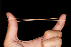
An experiment
Coils and Rubber bands
Coils and rubber bands have a natural size
If you apply a force to them, they expand
What is the relation between the expansion and the force?
Robert Hooke said it first
Robert Hooke (1635–1703) was an English natural philosopher, architect and polymath.
In 1660, Hooke discovered the law of elasticity which describes the linear variation of tension with extension
“The extension is proportional to the force”
Robert Hooke
Natural philosophy was the study of nature and the physical universe that was dominant before the development of modern science
Polymath (from Greek “having learned much”) is a person whose expertise spans a significant number of different subject areas
Biologist. Hooke used the microscope and was the fists to use the term cell for describing biological organisms.
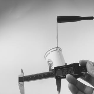
How do we model a coil?
The essence of the coil is:
It has a natural length \(L\)
If we change the length by \(x\), it pulls with a force \[\mathrm{force}(x)= K \cdot (L-x)\]
Remember that straight lines can be represented by the formula \[\text{n_marbles}=A+B\cdot \text{length}\] The coefficient \(A\) is the value where the line intercepts the vertical axis
The coefficient \(B\) is how muchlength goes up when n_marbles increases. This is called slope
Physical interpretation of the linear model
The formula from Hooke’s Law is \[\text{force}=K\cdot(L-\text{height})\] Since force is the weight of the balls, we can write \[-m g\cdot\text{n_balls}=K\cdot(L-\text{lenght})\] which can be re-written as \[\text{lenght}=\underbrace{L}_{A}+\underbrace{\frac{m g}{K}}_{B}\cdot\text{n_balls}\]
Physical interpretation of coef(model)
When there are no balls, the length of the coil is \(L\), in this case
coef(model)[1]
(Intercept)
   76.48188
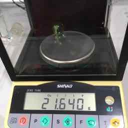
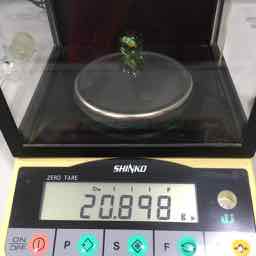
If the mass of each ball is 20gr, we can find \(K\) as


 Robert Hooke (1635–1703) was an English natural philosopher, architect and polymath.