Class 8: Vectors
Computing in Molecular Biology and Genetics 1
Andrés Aravena, PhD
2 November 2020
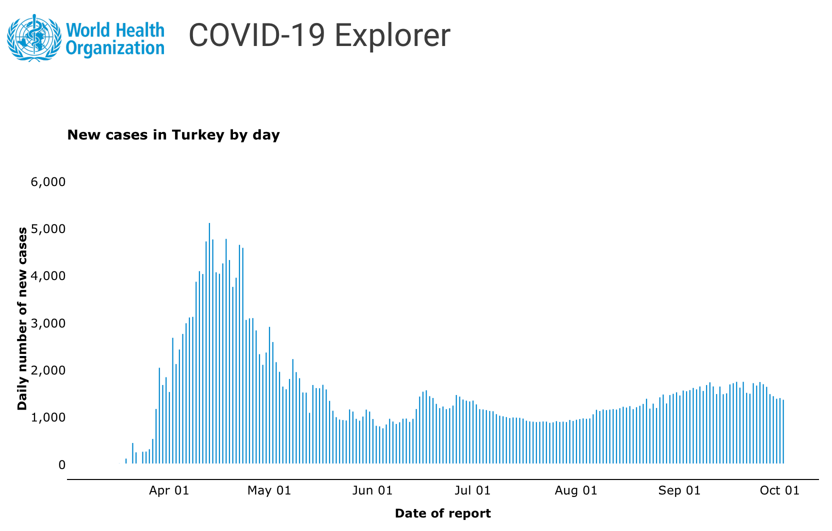
We want to make plots like this
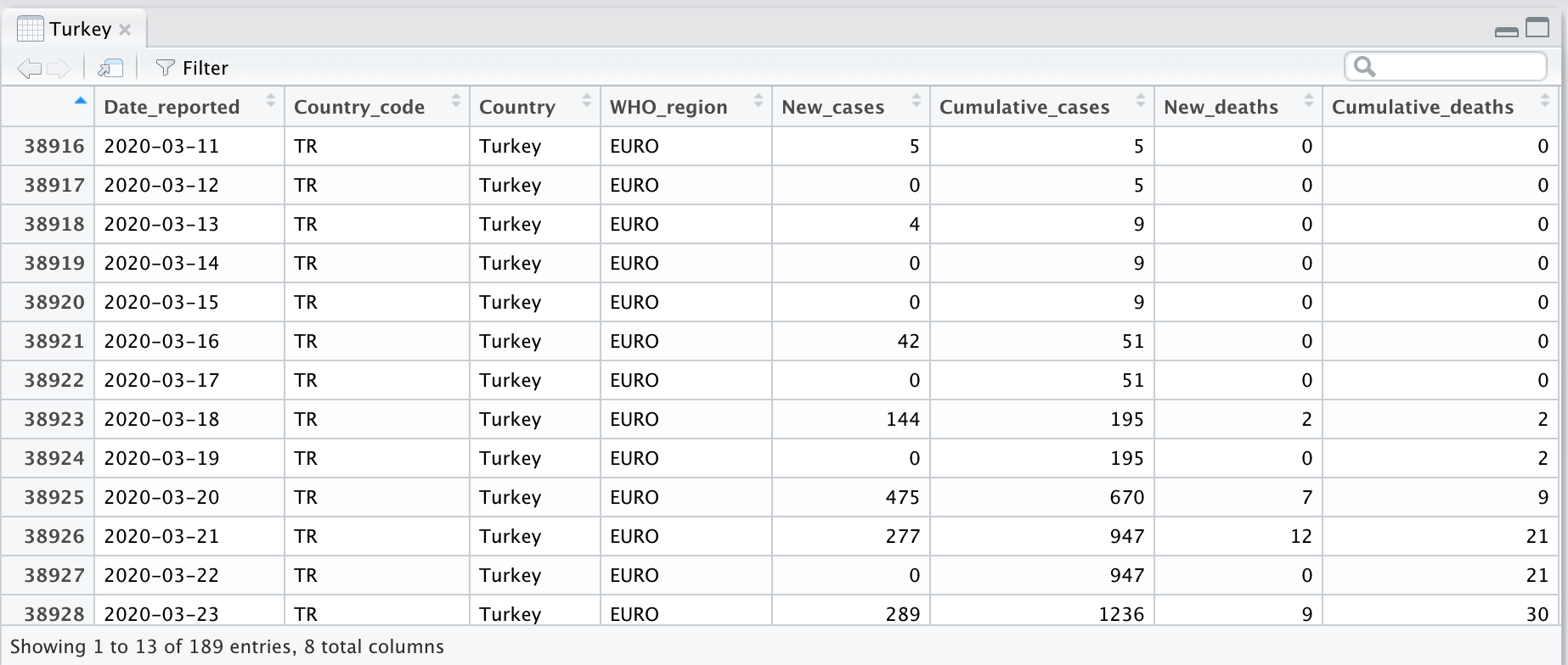
From data like this

Source: World Health Organization website
Structured in tables like this
Example
COVID-19 data
This is an Example
I will show you some commands to get real data in R
Follow all the steps carefully
We will explain the commands later
This example will show the possibilities
Download COVID-19 data from WHO
Open the webpage
https://covid19.who.int/WHO-COVID-19-global-data.csv
This is a text file
The extension .csv means “comma-separated values”
Save it in your computer
- Use the “Save…” option in your web browser
- You may need to right-click on the window
- Pay attention to the folder used to save the file
- Try to use
Downloads
- Try to use
- Open the file in R
- Environment → Import Dataset → From Text (base)…
One way to load data into R
Environment → Import Dataset → From Text (base)…

Find the file that you already downloaded
This will move data from the disk to the main memory
Change the name to covid

See the code in the console
The console shows the command used to read the file

Next time we can import data by writing this command
We can see covid on “Environment”
It is a big table, with thousands of rows

Lets make a table for Turkey
we will explain the commands later
Write the following commands in R
Be careful with UPPER and lower case
There are two = signs in the command
What do we have in Environment now?
There is a new table called Turkey
Let’s see one single column
  [1]    5    0    4    0    0   42    0  144    0  475  277    0  289
 [14]  293  343  561 1196 2069 1704 1869 1556 2704 2148 2456 2786 3013
 [27] 3135 3148 3892 4117 4056 4747 5138 4789 4093 4062 4281 4801 4353
 [40] 3783 3977 4674 4611 3083 3116 3122 2861 2357 2131 2392 2936 2615
 [53] 2188 1983 1670 1614 1832 2253 1977 1848 1546 1542 1114 1704 1639
 [66] 1635 1708 1610 1368 1158 1022  972  961  952 1186 1141  987  948
 [79] 1035 1182 1141  983  839  827  786  867  988  930  878  914  989
 [92]  993  922  987 1195 1459 1562 1592 1467 1429 1304 1214 1248 1192
[105] 1212 1268 1492 1458 1396 1372 1356 1374 1293 1192 1186 1172 1154
[118] 1148 1086 1053 1041 1024 1003 1016 1012 1008  992  947  933  926
[131]  918  924  931  928  902  913  937  921  927  919  963  942  967
[144]  982  996  987  995 1083 1178 1153 1185 1172 1182 1193 1183 1212
[157] 1243 1226 1256 1192 1233 1263 1303 1412 1203 1309 1217 1443 1502
[170] 1313 1491 1517 1549 1482 1587 1572 1596 1642 1612 1673 1578 1703
[183] 1761 1673 1512 1671 1509 1527 1716
This is what we call a vector in R
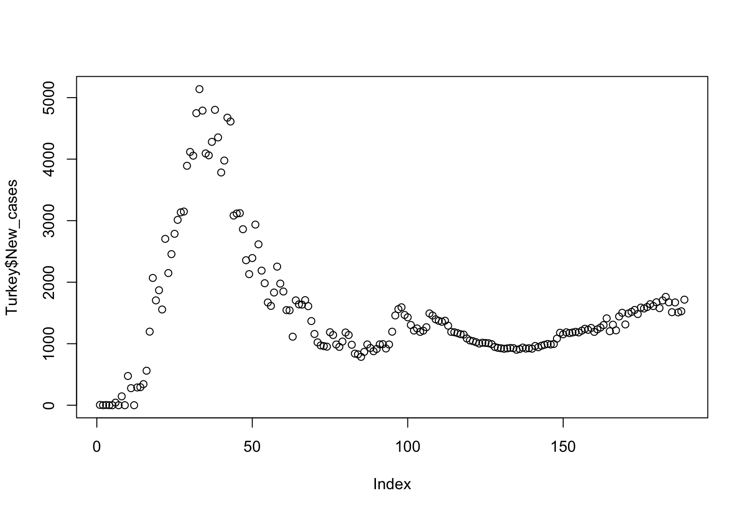
Now we can draw a plot
Vectors
Variables can store several values
In the previous class we used variables to store single numbers
It is useful to handle several values at the same time, all grouped in the same variable
Vectors
The most simple objects in R
Group of values, all with the same type
For example, a set of numbers
[1] 2392 2936 2615 2188 1983 1670 1614 1832 2253 1977 1848Vectors are a data structure
The structure of a variable corresponds to the way the data is organized
Vectors are the simplest way to organize data
We will learn others later
Functions over vectors
In the previous cases we saw functions that work on a single number
[1] 3Now we will use functions working on a vector
Functions over vectors
vector to number
length(): Number of elements in the vector
[1] 189sum(): Total of all values in the vector
[1] 292878Functions over vectors
vector to number
min(): smallest value
[1] 0max(): largest value
[1] 5138Two kinds of average
vector to number
mean(): mean value
[1] 1549.619median(): median value
[1] 1233Basic statistics
vector to number
var(): variance
[1] 1074685sd(): standard deviation
[1] 1036.67Question
What happens if you use sqrt() over a vector?
Creating vectors
Simple concatenation
The function c() (“concatenate”) takes many values and makes a single vector
[1] 1 2 3[1] 10 20Concatenation means “to put in the same chain”
Storing vectors in variables
We use the <- operator for assignment.
Now we look inside the variables
[1] 1 2 3[1] 10 20Vectors can also be concatenated
Variables x and y are two vectors
We can concatenate them into a larger vector
[1] 1 2 3 10 20 5A number is a vector of size 1
If the vector has only one element,
you do not need to use c()
Instead of c(3) just write 3
Other ways to create vectors
Repetitions
A common case is a vector with the same value repeated several times
For that case, we use the rep() function
[1] 1 1 1The first input of rep() is the value to repeat
The second is how many times to repeat
rep() can work with vectors
The first input can be a vector
[1] 7 9 13 7 9 13 7 9 13 7 9 13The complete vector is repeated
Second input can also be a vector
Both vectors must have the same length
[1] 7 7 9 13 13 13Each element of the first vector is repeated according to the value in the second vector
Sequences
A vector with numbers between 4 and 9
[1] 4 5 6 7 8 9 10 11 12 13 14 15 16 17 18 19 20Two numbers separated by :
results in a vector from the first up to the second
a:b becomes c(a, a+1, a+2, …, b)
Another way to write a:b
A vector with numbers between 4 and 20
[1] 4 5 6 7 8 9 10 11 12 13 14 15 16 17 18 19 20This is the same as 4:20
It is easier to write using :
Advantage of seq() function
We can go from 4 to 10 incrementing by 2
[1] 4 6 8 10 12 14 16 18 20The function can take an extra input
But it is hard to remember the meaning
Function inputs have names
Instead of
[1] 4 6 8 10 12 14 16 18 20we can write
[1] 4 6 8 10 12 14 16 18 20seq() is more flexible
We can say how many numbers we want, instead of the last value
[1] 4 5 6 7 8 9 10 11 12 13 14 15seq() is more flexible
seq() fills the missing inputs
[1] 4.0 4.5 5.0 5.5 6.0Learn more in the Help page
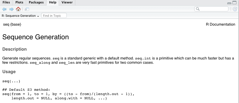
How to use functions
The inputs are inside round parenthesis
Their role given by position or by name
If the input is optional, then you must write its name
The help page shows what is the default value
Arithmetic with vectors
Take two same-length vectors
[1] 1 2 3 4 5 6 7 8[1] 2 5 8 11 14 17 20 23(this is just an example)
Arithmetic of vectors and vectors
[1] 3 7 11 15 19 23 27 31[1] -1 -3 -5 -7 -9 -11 -13 -15[1] 2 10 24 44 70 102 140 184Works component by component
Arithmetic of vectors and numbers
[1] 3 4 5 6 7 8 9 10[1] -1 0 1 2 3 4 5 6[1] 2 4 6 8 10 12 14 16Again, component by component
Component by component
We can make new vectors by combining
- two vectors of the same length
- one vector and a single number
- That is, with a vector of length 1
Question: What happens if the vectors do not have the same length?
Summary
- We can create vectors with
c(),rep(), andseq() a:bis the shorthand ofseq(from=a, to=b)- We can read vectors from files (more detail later)
- We can use functions over vectors
- Some functions give another vector
- Some functions give a number
- We can do arithmetic with vectors
- vector with vector, same length
- vector with number