What is the question?

We want to know

• Which genes are being expressed
• How much of each gene is being expressed
• How does expression change
  • In time
  • Under different conditions
  • Between strains/mutants/cell lines

The Big Assumption

Measuring protein concentration is hard

We assume that protein concentration is proportional to mRNA concentration

• Which genes are being transcribed
• How much of each gene is being transcribed
• How does transcription change
  • In time
  • Under different conditions
  • Between strains/mutants/cell lines

qPCR

If you have primers for each gene

• specific to each gene
• thermodynamically stable
• efficient

Raw data: CT value for each gene/condition
and CT value for calibration reference

Hybridization methods

Southern/Northern/Western blot can detect, but not quantify
(I think so. I’m not a biologist)

Instead, we have macro- and microarrays

Raw data: Light intensity (luminescence) in one or more wave length

This is measured in arbitrary units, and is a number between 0 and 65536
(that is, a 16-bits value)

Problem: it is hard to compare genes

• Light intensity depends on hybridization rate
• Hybridization depends on oligo thermodynamics
  • GC content can have a big effect
• secondary structure blocks hybridization

Solution

Compare each gene with itself in a different condition

In other words, evaluate differential expression

• we cannot compare gene expression between genes
• we can compare differential gene expression between genes

RNAseq

mRNA is retro-transcribed and fragmented.
Fragments are sequenced. Reads are aligned to reference genome

Raw data: SAM/BAM file with location of each read in the reference genome

Processed data: Number of reads per gene

Problem: it is hard to compare genes

• longer genes get more reads
• different conditions get different number of reads

Solution 1: Normalization

• Divide by library size
• Divide by gene size

Normalization: RPKM, FPKM

Reads per kilobase per million:

• Count reads in a sample
  • divide that number by 1E6 (“per million”)
• Divide the read counts by the “per million” scaling factor
  • This normalizes for sequencing depth
  • We get reads per million (RPM)
• Divide the RPM values by the length of the gene, in kilobases
• This gives you RPKM.

FPKM is the same, but with fragments instead of reads

Normalization: TPM

Transcripts per million: similar to RPKM and FPKM
Just a different order of operations

• Divide the read counts by the length of each gene in kilobases
  • This gives reads per kilobase (RPK)
• Count up all the RPK values in a sample and divide this number by 1E6
  • This is “per million” scaling factor.
• Divide the RPK values by the “per million” scaling factor
  • This gives TPM

Solution 2

Compare each gene with itself in a different condition

In other words, evaluate differential expression

• we cannot compare gene expression between genes
• we can compare differential gene expression between genes

Differential Expression

Let’s say we have two conditions:

• wild-type cells
• mutant cells

Let’s take wild type as the base condition.

Fold change

For a given gene G, we want to calculate \[\frac{\text{Expression}(M)}{\text{Expression}(WT)}\]

This would be a number between 0 and ∞

When the gene is under-expressed, we get something between 0 and 1

When it is over-expressed, we get something between 1 and ∞

Log fold change

It is better to have a symmetrical result \[\log_2 \left(\frac{\text{Expression}(M)}{\text{Expression}(WT)}\right)\]

We use base 2 to get fold-change

• Positive numbers indicate over-expression
• Negative numbers indicate under-expression
• Zero indicates no-change

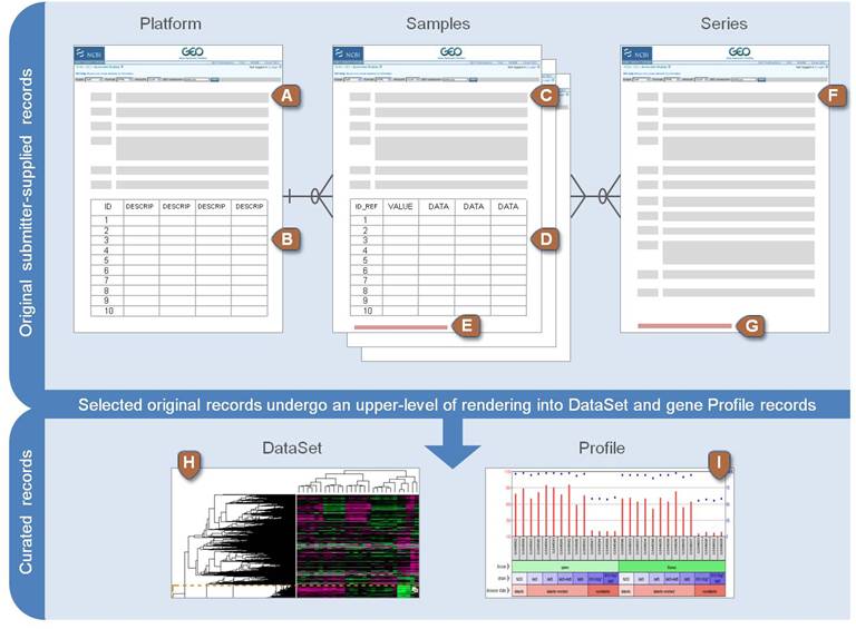
Data source: NCBI GEO

Gene Expression Omnibus

• Platforms
• Samples
• Series
• Data Set
• Profile

NCBI GEO data structure

Application: gene expression analysis

Let’s analyze gene_expression.csv

Each column is a gene, each row is a sample, taken from NCBI GSE95670. The values are absolute expression, we want to know

• The fold-change in expression
• If that change is real, or just noise

Factors indicate the condition

• The first three rows are mutants
• The last three rows are wild-type, or control

We can add a column with a factor describing the condition

m$condition <- factor(
    rep(c("Mutant", "Control"), c(3, 3)),
    levels=c("Control","Mutant"))

Now we can do a model for each gene

We want to measure fold-change. That means, we want to calculate log_2_(mutant/wild type)

gene_model <- lm(log2(LOC100652730) ~ condition, data=m)
gene_model

Call:
lm(formula = log2(LOC100652730) ~ condition, data = m)

Coefficients:
    (Intercept)  conditionMutant  
         7.2767           0.2465  

Confidence intervals

confint(gene_model)

                     2.5 %   97.5 %
(Intercept)      6.6628636 7.890598
conditionMutant -0.6216828 1.114595

Check if the confidence interval contains 0

Other cases

lm(log2(IZUMO4) ~ condition, data=m) %>% confint(parm = "conditionMutant")

                    2.5 %   97.5 %
conditionMutant 0.5694141 3.608096

lm(log2(RHOU) ~ condition, data=m) %>% confint(parm = "conditionMutant")

                    2.5 %     97.5 %
conditionMutant -1.433264 -0.2166465

lm(log2(STC1) ~ condition, data=m) %>% confint(parm = "conditionMutant")

                  2.5 %   97.5 %
conditionMutant 4.45331 8.712368

lm(log2(PDGFC) ~ condition, data=m) %>% confint(parm = "conditionMutant")

                    2.5 %    97.5 %
conditionMutant -4.362937 -2.184466