Class 13: DNA Sequencing and Genome Assembly
Bioinformatics
Andrés Aravena
January 8, 2021
What to sequence
What to sequence
In broad terms there are three alternatives
- PCR products a.k.a. amplicons
- Random genomic fragments a.k.a shotgun
- RNA messengers
Amplicons
- highly targeted
- enables analysis of genetic variation in specific regions
- uses primers targeted to regions of interest
- useful for the discovery of mutations in complex samples
- such as tumors mixed with germline DNA
- used in sequencing the 16S rRNA gene in metagenomics
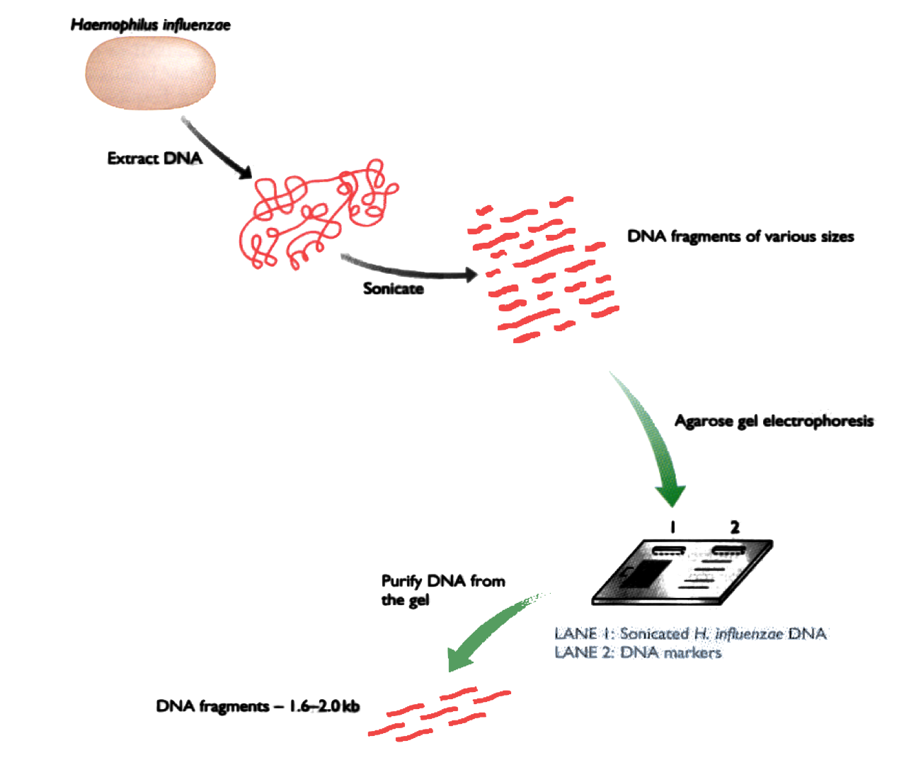
Shotgun DNA Sequencing
RNA sequencing
- Reverse transcription into cDNA
- Easier when there is a poly-A tail
- Usually the genome is known, and we care only about measuring gene expression
- If the genome is unknown, the mRNA gives us a good part of the genome
- That strategy is called expressed sequence tags (EST)
Fragments v/s reads
In all these cases we get a DNA fragment, about a few thousands bp long (let’s say 500–5000bp)
Each fragment is a physical object
Each strand can be sequenced and produce a read
Usually we have two reads for each fragment
They are sometimes called “forward” and “reverse” reads
How sequencing works
DNA sequencing
There are many sequencing methods, based on different physicochemical properties
- activity of restriction enzymes
- florescence
- electronic properties of nucleotides
- chemistry of DNA duplex formation
They are in constant development. We will focus on their key properties
See DNA sequencing on the WikiPedia for more details
Broadly speaking
- Sanger method: few short reads
- NGS: many very short reads
- 3rd generation: few long reads
Idea of Sanger method
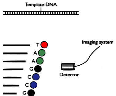
DNA is separated in 4 parts, each part is mixed with a different restriction enzyme. Then the fragments are separated by electrophoresis.
In a second version, each part is marked with a different fluorophores and then placed in a single capilar electrophoresis, with a light detector
Sanger requires cloning

Cloning vector

- know restriction-enzyme cut sites
- known binding-sites for primers
- antibiotic-resistance genes
- replication origin site
Part of the vector will be sequenced in every read
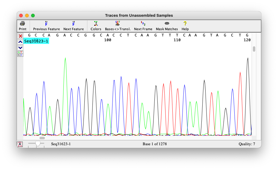
Sanger method’s result
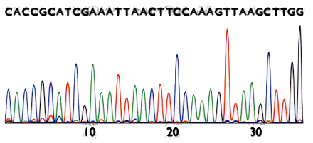
The result is a chromatogram. Filenames ending in .AB1 or .SCF
New generation sequencing
- Roche 454
- Illumina Solexa
- Ion Torrent
- ABI SOLID
Third generation
- DNA nanoball
- Pacific Biotech (PacBio)
Roche 454
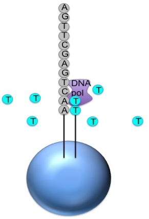
Generic adaptors are added to the ends and annealed to beads, one DNA fragment per bead
The fragments are then amplified by PCR
Each bead is placed in a single well of a slide
Each well will contain a single bead, covered in many PCR copies of a single sequence
The slide is flooded with one of the four NTP species
Roche 454
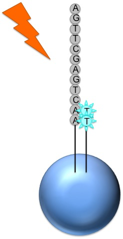
The nucleotide is incorporated when it matches the template
If that single base repeats, then more will be added
The addition of each nucleotide releases a light signal, and is registered with a hight resolution video
Roche 454
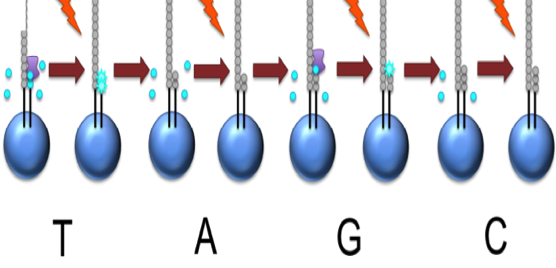
This NTP mix is washed away
The next NTP mix is now added and the process repeated, cycling through the four NTPs.
This kind of sequencing generates graphs for each sequence read, showing the signal density for each nucleotide wash
The sequence can then be determined computationally from the signal density in each wash.
Roche 454
Sequencing by synthesis
can sequence 0.7 gigabase per run
run time 23 hours
read length 700-800 bases
Illumina Solexa
also sequencing by synthesis
- old model Genome Analyzer can sequence 1Gb per run
- Solexa model can sequence 600 Gb per run
- HiSeq model 100 bases read length average 30Gb per run
- 11 day in regular mode
- 2 day in rapid run mode
Illumina Solexa
over 70% of the market
- ∼$1000 MiSeq
- ∼$3000 HighSeq
- ∼ 1.5 days
Illumina Solexa
- output of sequencing data per run: 600 Gb
- read lengths: approximately 100 bp
- cost is cheap
- run times are long: 3-10 days
ABI-SOLID
Sequencing by ligation
Supported Oligonucleotide Ligation and Detection (SOLiD)
- Solid 4 model can read 80-100 Gb per run (coverage 30Gb)
- average read length 50 bases
- fragment length 400-600-bp
ABI-SOLID
The advantage of this method is accuracy with each base interrogated twice
Major disadvantages
- short read lengths (50–75 bp)
- very long run times of 7 to 14 days
- need for computational infrastructure and expert computing personnel for analysis of the raw data
Ion torrent
- Developed by the inventors of 454 sequencing
- With two major changes.
- nucleotide sequences are detected electronically by changes in the pH of the surrounding solution rather than by the generation of light
- sequencing reaction is performed in a microchip with flow cells and electronic sensors on each cell
- The incorporated nucleotide is converted to an electronic signal
PacBio
- PacBio model RS II produces average read lengths over 10 kb, with an N50 of more than 20 kb and maximum read lengths over 60 kb
- Error rate of a continuous long read is relatively high (around 11%–15%)
- The error rate can be reduced by generating circular consensus sequences reads with sufficient sequencing passes.
Summary
| Method | Read length (bp) | Error rate (%) | No. of reads per run | Time per run | Cost per million bases (USD) |
|---|---|---|---|---|---|
| Sanger ABI 3730x1 | 600-1000 | 0.001 | 96 | 0.5–3 h | 500 |
| Illumina HiSeq 2500 (Rapid Run) | 2 × 250 | 0.1 | 1.2 × 10⁹ (paired) | 1–6 days | 0.04 |
| PacBio RS II: P6-C4 | 1.0–1.5 × 10⁴ | 13 | 3.5–7.5 × 10⁴ | 0.5–4 h | 0.4–0.8 |
| Oxford Nanopore MinION | 2–5 × 10³ | 38 | 1.1–4.7 × 10⁴ | 50 h | 6.44–17.9 |
Base calling
From chromatograms to sequences
Sequencers produce signals
- Sanger produces chromatograms
- Pyrosequencing make videos
- others
each method has their own tool to call the bases
For Sanger, that tool is called Phred
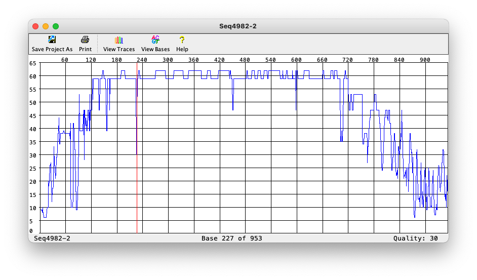
Phred
Phred quality
Signal–Ratio is different for each base
As usual we use logarithms, multiply by a constant, and take the integer part \[\lfloor10\cdot\log_{10}(\text{Signal}/\text{Noise})\rfloor\]
Phred quality
| Q | Error.probability | Probability.of.correct |
|---|---|---|
| 10 | 0.1000000 | 0.9000000 |
| 15 | 0.0316228 | 0.9683772 |
| 20 | 0.0100000 | 0.9900000 |
| 30 | 0.0010000 | 0.9990000 |
| 40 | 0.0001000 | 0.9999000 |
| 50 | 0.0000100 | 0.9999900 |
| 60 | 0.0000010 | 0.9999990 |
| 70 | 0.0000001 | 0.9999999 |
| 80 | 0.0000000 | 1.0000000 |
Phred quality of each base
Phred file format (.phd)
BEGIN_SEQUENCE GTFAG75TF.scf

BEGIN_COMMENT

CHROMAT_FILE: GTFAG75TF.scf
ABI_THUMBPRINT: 0
TRACE_PROCESSOR_VERSION:
BASECALLER_VERSION: phred 0.071220.c
PHRED_VERSION: 0.071220.c
CALL_METHOD: phred
QUALITY_LEVELS: 99
TIME: Fri Nov 22 15:00:37 2019
TRACE_ARRAY_MIN_INDEX: 0
TRACE_ARRAY_MAX_INDEX: 9116
TRIM: 34 555 0.0500
TRACE_PEAK_AREA_RATIO: 0.0255
CHEM: prim
DYE: rhod

END_COMMENT

BEGIN_DNA
g 6 8
a 6 24
g 6 28
a 8 45
g 8 50
a 8 59
t 8 77
c 8 87
t 9 100
a 9 115
g 11 124
t 11 140
g 15 147
t 8 162
g 9 170
c 12 182
t 9 197
g 17 207
g 20 221
a 21 234
Files of type .qual
This is FASTA format, with numbers instead of letters
Each number is the quality of the corresponding letter
>GTFAG75TF.scf    702      0    702  SCF
6 6 6 8 8 8 8 8 9 9 11 11 15 8 9 12 9 17 20 21 20
18 9 10 6 6 6 6 8 16 11 6 6 8 20 17 30 30 44 44 29
16 9 9 9 22 23 44 44 32 32 32 34 34 34 38 38 38 38
34 38 38 38 38 44 34 34 34 39 44 47 47 53 53 53 53
53 47 47 47 47 47 47 53 53 47 53 53 53 47 59 59 59
59 59 59 59 59 59 59 59 59 59 59 59 59 59 59 59 59
59 59 59 59 59 59 59 59 59 59 59 24 24 59 59 59 59
62 62 62 62 62 62 62 59 59 59 59 59 59 51 59 59 62
59 59 59 59 59 59 59 59 56 59 59 59 59 59 56 56 56
39 38 38 38 56 56 56 56 59 62 62 62 62 59 59 59 59
59 59 59 62 62 62 62 62 62 44 40 40 28 28 28 59 59
56 59 59 56 56 56 56 59 56 56 59 59 59 59 59 59 59
59 56 56 56 56 56 56 59 59 59 59 62 59 59 56 56 56
59 56 59 59 59 59 59 59 47 59 59 59 59 59 59 59 59
59 59 59 59 59 56 56 56 56 56 59 62 59 59 59 59 59
59 59 59 59 59 59 59 62 62 62 62 59 59 59 59 59 59
59 59 59 59 59 59 59 59 59 59 59 59 59 59 59 59 59
25 25 59 59 59 59 59 59 59 59 59 59 59 59 59 59 59
59 53 53 43 43 43 53 53 53 53 53 53 53 53 53 53 47
47 47 47 47 44 39 53 39 39 39 39 39 53 53 53 53 53
47 47 43 44 38 38 32 38 27 27 32 31 29 29 35 35 36
35 35 38 38 43 43 43 38 53 39 34 34 53 53 47 43 47
53 53 53 53 53 53 47 47 43 39 32 32 29 30 30 38 34
35 26 44 44 44 38 33 26 24 27 29 33 33 35 38 38 38
34 34 34 38 32 38 34 34 34 39 32 39 34 30 32 32 34
34 38 38 38 38 38 38 38 38 29 29 27 18 17 27 27 27
20 20 33 29 33 32 32 32 35 38 38 34 34 34 35 47 34
38 32 32 25 27 20 20 15 24 30 32 32 32 31 29 29 27
29 32 31 24 29 33 32 33 31 28 29 29 24 24 29 29 29
32 32 31 29 24 29 24 24 23 19 20 23 21 21 17 18 10
10 10 9 7 9 9 9 9 11 19 25 21 21 20 23 24 24 24 18
18 10 10 10 18 20 20 14 24 15 20 20 29 24 17 20 15
14 14 12 11 9 8 6 6 6 8 8 8 10 10 10 18 18 24 24 16
18 13 11 11 14 10 9 16 11 10 10 11 10 13 10 19 21
17 8 6 6 6 11 10 11 11 10 10 12 10 19 18 9 7 10 6
6 6 9 11 9 10 10 12 8 6 6 6 6 8 8 9 9 9 9 8 11 11
11 7 7 11 6 6 6 6 6 6 9 7 6 6 8 8 11 6 6 6 6 6 6 6
9 6 6 6 8 6 8 9 8 6 6 6 6 6 9 6 6 8 6 6 6 6 6 8 11
12 11 9 9 9 7 12 8 9 7 9 9 9 6 6 9 9 7 7 7 7
FASTQ
Inspired by FASTA, combining sequences and qualities
- Each entry starts with
@instead of>, and the read ID - The second line is the sequence, base by base
- Line 3 starts with
+, can be followed by the ID again - Line 4 has the qualities encoded, one symbol for each base
@001043_1783_0863
CTGATCATTGGGCGTAAAGAGTGCGCAGGCGGTTTGTTAAGCGAGATGTGAAAGCCCCGGGCTCAACCTGGGAATTGCATTTCGAACTGGCGAACTAGAGTCTTGTAGAGGGGGTAGAATTCCAGGTGTAGCGGTGAAATGCGTAGAGATCTGGAGGAATACCGGTGGCGAAGGCGGCCCCCTGGACAAAGACTGACGCTCAGGCACGAAAGCGTGGGGAGCAAACAGGATTAAATACCCTCGTA
+001043_1783_0863
<<<<<<<>;>=0<<<=<-<<<<<<<<<>:<>:>=/<?;?;<<<<<<<<<<>=0<<<5(=<-<<<>;?;<>=0>;?;<<<>=/<<>:;<<8<<?;<<<:<<<<?;<<<<<;:71(;;;?;>9>:<>:;<<<;<>9<<>=1<<<<<<<<<<<<<>;;?;>:<:?;?;<>:<<?;?;<?;;;70';>;9<>=1;:<;;;:<<<<<?;;<<<>=2<<;<<<5(<;9>=0;<?;<>;=<2:8>=1:9<<9
Encoding quality in a single letter
Each quality value between 0 and 90 is represented by the corresponding symbol in the following text
!"#$%&'()*+,-./0123456789:;<=>?@ABCDEFGHIJKLMNOPQRSTUVWXYZ[\]^_`abcdefghijklmnopqrstuvwxyz{|}~Initially FASTQ were supposed to have sequences and qualities in several lines, but the symbols + and @ can be quality values
To avoid ambiguity, each entry has exactly 4 lines.
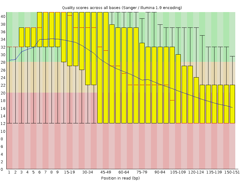
Quality control: FastQC
Assembly
Assembling genomes
Once we have all the reads, how do we get the genome?
Imagine a book of 1000 pages:
- several copies of the book are cut randomly in one million pieces
- different pieces may overlap
- half of the pieces are lost
- the remaining half is splashed with ink in the middle
The problem is to reconstruct the original book
When not to assemble
If we already know the genome, we do not need to assemble it
This is obvious. Still, it is an important case
- When we sequence expressed genes, i.e. RNAseq
- When we look for polymorphisms
De novo Strategies
Also called ab initio, these are Latin words meaning “from new” or “from the start”
There are basically three strategies used to assemble genomes
- Greedy algorithms
- Overlap – Layout – Consensus
- De Bruijn graphs
Today we will speak about the first two strategies
Greedy algorithm
Given a set of sequence fragments, the object is to find a longer sequence that contains all the fragments.
- Evaluate the pairwise alignments of all fragments
- Choose two fragments with the largest overlap
- Merge the chosen fragments
- Repeat step 2 and 3 until only one fragment is left.
Overlap
- All reads are compared to each other
- and to their reverse-complement
- The alignment considers each base’s quality
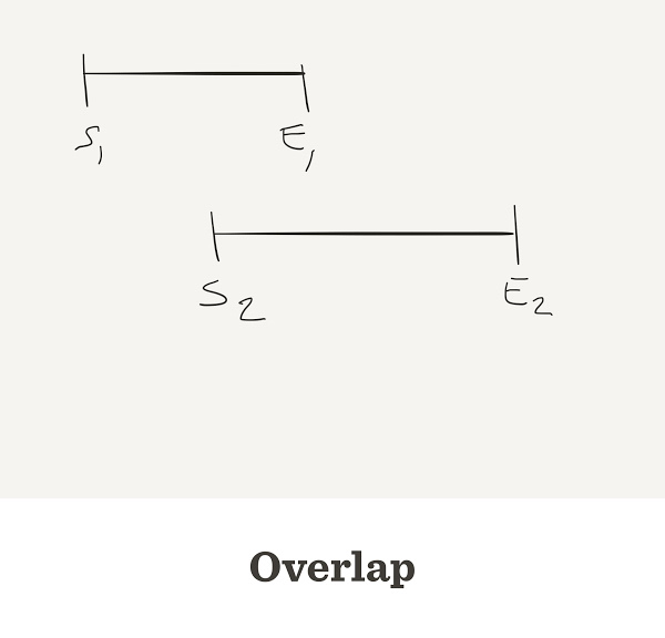
- When the end of one read matches the start of another read, we say that they overlap
Sometimes reads do overlap
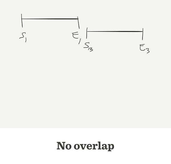
Sometimes they do not overlap
Problems with the greedy approach
The final sequence may be wrong
Two different reads A, B may match the same read X
To decide which one is correct, a Layout stage is used
Layout
In this approach, the overlap between reads is used to build a graph of reads relationships
This graph determines the layout of all reads,
that is, their relative positions
Contigs
Usually there are several independent groups of reads that are not connected in the layout graph
(we say that the graph has several connected components)
All the reads that are connected together form a contig
Consensus
Once the layout is clear, the last step is to retrieve the consensus sequence of the contig
In fact, it is not a consensus. It is a vote. The majority wins
High quality votes are more important than low quality ones
Example: Phrap assembler
The human genome project used Phred for base-calling and Phrap for assembly
Phrap produces several files. The most important has extension .ace
These programs are free for academic usage (non-commercial)
Example ACE file
AS 36 39

CO Contig1| 131 1 1 U
gctagaaaaaaaaggactcccagtagaaatacgtacaataaagtaggttc
ctctagttaactgttacaaaataagtttcccattggtaatataatagatt
tataactgttatatccagagcaacctagggg

BQ
 15 15 15 15 15 15 15 15 15 15 15 15 15 15 15 15 15 15 15 15 15 15 15 15 15 15 15 15 15 15 15 15 15 15 15 15 15 15 15 15 15 15 15 15 15 15 15 15 15 15
 15 15 15 15 15 15 15 15 15 15 15 15 15 15 15 15 15 15 15 15 15 15 15 15 15 15 15 15 15 15 15 15 15 15 15 15 15 15 15 15 15 15 15 15 15 15 15 15 15 15
 15 15 15 15 15 15 15 15 15 15 15 15 15 15 15 15 15 15 15 15 15 15 15 15 15 15 15 15 15 15 15

AF 5765593 U 1
BS 1 131 5765593

RD 5765593 131 0 6
gctagaaaaaaaaggactcccagtagaaatacgtacaataaagtaggttc
ctctagttaactgttacaaaataagtttcccattggtaatataatagatt
tataactgttatatccagagcaacctagggg
Example ACE file (last part)
CO Contig36 111 2 63 U
taTAAAGTCGATGGGGAGGAAGATAGGGGAGCTAAAGCCATAGGGAAACC
ACGTAGTTCTGCGTCAAGCGTTgccttcCGAGGTGCTCTCCGCTTTTCCA
TGCtccaatcg

BQ
 15 15 25 25 25 25 25 25 25 25 25 25 25 25 25 25 25 25 25 25 25 25 25 25 25 25 25 25 25 25 25 25 25 25 25 25 25 25 25 25 25 25 25 25 25 25 25 25 25 25
 25 25 25 25 25 25 25 25 25 25 25 25 25 25 25 25 25 25 25 25 25 25 15 15 15 15 15 15 25 25 25 25 25 25 25 25 25 25 25 25 25 25 25 25 25 25 25 25 25 25
 25 25 25 15 15 15 15 15 15 15 15

AF 5648323 U 1
AF 5703145 U 1
Depth

Online Material
Indiana University Bloomington, “Introduction to Bioinformatics”, Lecture by Yuzhen Ye
Université Lyon I, Network Algorithms for Molecular Biology lesson on “Introduction to (de novo) assembly”, by Blerina Sinaimeri
MIT, “Foundations of Computational Systems Biology”, Lecture by David K. Gifford