Class 11: Finding Binding Sites
Bioinformatics
Andrés Aravena
25 December 2020
Where are we?
Big picture: Bioinformatics
- What are the questions
- What are the tools
- What are the inputs and outputs
- What are the file types
- How to use the tools
- Web tools
- Command line tools
- How to make your own tools
- BioPython
- BioConductor in R
- How to understand the results
Big picture: This course
- Finding data online
- Taxonomy
- Pairwise Alignment
- Multiple Alignment
- Phylogenetic Trees
- DNA sequencing
- Genome Assembly
- Functional Annotation
- Finding Binding Sites
- Primer design
- Gene expression analysis
Big picture: Mathematics for Biologists
- Logic
- Sets
- Relationships
- Clustering
- Complexity
- Graphs/Networks
- Probabilities
Big picture: Combined
- Finding data online (Sets, Logic)
- Taxonomy (Relationships)
- Pairwise Alignment (Sets, Probability)
- Multiple Alignment (Complexity)
- Phylogenetic Trees (Clustering)
- DNA sequencing (Probabilities)
- Genome Assembly (Graphs)
- Functional Annotation (Graphs, Probs)
- Finding Binding Sites (Probabilities)
- Primer design (Probabilities)
- Gene expression analysis (Probabilities)
Finding Binding Sites
Three kinds of Proteins
Broadly speaking, there are three kinds of proteins
- Structural pieces:
- keratine (hair), tubuline (tubes)
- Enzymes:
- catalyzers that trigger chemical reactions
- transform one metabolite into another
- Information handlers:
- replication
- transcription factors
- translation
Transcription factors
Transcription Factors (TF) are proteins that can bind to DNA
The binding sites of a TF are the places in the genome where the TF binds
They are short regions (about 20bp long)
One protein can bind in several sites
We want to see what do these site have in common
Some sites are identified
Experiments can give us the sequence where a TF binds
For example, the E.coli protein Fnr binds in sites like this:
TTGATCGTTATCAA
TTGATTTACATCAA
ATGATAAATATCAA
TTGAGGTAGGTCAA
TTGATTTGGATCAC
TTGATCTCACCCGG
TTGATTAACATCAA
See http://http://www.prodoric.de/matrix.php?matrix_acc=MX000004
Motif: what all sites have in common
There are tens of binding sites for each TF
We can align them to see what is conserved
We can summarize all of them counting each nucleotide on every column
That is, calculating the frequency of each nucleotide
Absolute Frequency Matrix
| 1 | 2 | 3 | 4 | 5 | 6 | 7 | 8 | 9 | 10 | 11 | 12 | 13 | 14 | |
|---|---|---|---|---|---|---|---|---|---|---|---|---|---|---|
| A | 3 | 0 | 1 | 24 | 2 | 9 | 6 | 15 | 7 | 23 | 5 | 2 | 27 | 25 |
| C | 1 | 0 | 1 | 3 | 0 | 7 | 4 | 5 | 8 | 4 | 3 | 26 | 1 | 4 |
| G | 1 | 2 | 30 | 2 | 4 | 3 | 3 | 3 | 5 | 4 | 1 | 3 | 1 | 2 |
| T | 27 | 30 | 0 | 3 | 26 | 13 | 19 | 9 | 12 | 1 | 23 | 1 | 3 | 1 |
Let’s give a name to this matrix. It is \(F.\) \[\begin{aligned} F(“A”, 1) & =3\\ F(“T”, 1) & =27\\ F(“C”, 6) & =7 \end{aligned} \]
What do we see here?
| 1 | 2 | 3 | 4 | 5 | 6 | 7 | 8 | 9 | 10 | 11 | 12 | 13 | 14 | |
|---|---|---|---|---|---|---|---|---|---|---|---|---|---|---|
| A | 3 | 0 | 1 | 24 | 2 | 9 | 6 | 15 | 7 | 23 | 5 | 2 | 27 | 25 |
| C | 1 | 0 | 1 | 3 | 0 | 7 | 4 | 5 | 8 | 4 | 3 | 26 | 1 | 4 |
| G | 1 | 2 | 30 | 2 | 4 | 3 | 3 | 3 | 5 | 4 | 1 | 3 | 1 | 2 |
| T | 27 | 30 | 0 | 3 | 26 | 13 | 19 | 9 | 12 | 1 | 23 | 1 | 3 | 1 |
Each column has the same total
This matrix was built with 32 sequences
There are no gaps in the alignment
The sum of each column is 32. That is, \[\forall j\qquad \sum_{X\in \{A,C,G,T\}} F(X, j)=32\]
Other TF may have more or less sequences
To compare equal to equal, we divide everything by 32
Each column has the same total
This matrix was built with 32 sequences
There are no gaps in the alignment
The sum of each column is 32. That is, for each \(j\) we have \[F(“A”,j)+ F(“C”,j)+ F(“G”,j)+ F(“T”,j)=32\]
Other TF may have more or less sequences
To compare equal to equal, we divide everything by 32
Relative Frequency Matrix
| 1 | 2 | 3 | 4 | 5 | 6 | 7 | 8 | 9 | 10 | 11 | 12 | 13 | 14 | |
|---|---|---|---|---|---|---|---|---|---|---|---|---|---|---|
| A | 0.09 | 0.00 | 0.03 | 0.75 | 0.06 | 0.28 | 0.19 | 0.47 | 0.22 | 0.72 | 0.16 | 0.06 | 0.84 | 0.78 |
| C | 0.03 | 0.00 | 0.03 | 0.09 | 0.00 | 0.22 | 0.12 | 0.16 | 0.25 | 0.12 | 0.09 | 0.81 | 0.03 | 0.12 |
| G | 0.03 | 0.06 | 0.94 | 0.06 | 0.12 | 0.09 | 0.09 | 0.09 | 0.16 | 0.12 | 0.03 | 0.09 | 0.03 | 0.06 |
| T | 0.84 | 0.94 | 0.00 | 0.09 | 0.81 | 0.41 | 0.59 | 0.28 | 0.38 | 0.03 | 0.72 | 0.03 | 0.09 | 0.03 |
Let’s call this matrix with the name \(f.\) We have \[\forall X, \forall j\qquad f(X, j)=\frac{F(X, j)}{\sum_Y F(Y, j)}\]
Relative Frequency Matrix
| 1 | 2 | 3 | 4 | 5 | 6 | 7 | 8 | 9 | 10 | 11 | 12 | 13 | 14 | |
|---|---|---|---|---|---|---|---|---|---|---|---|---|---|---|
| A | 0.09 | 0.00 | 0.03 | 0.75 | 0.06 | 0.28 | 0.19 | 0.47 | 0.22 | 0.72 | 0.16 | 0.06 | 0.84 | 0.78 |
| C | 0.03 | 0.00 | 0.03 | 0.09 | 0.00 | 0.22 | 0.12 | 0.16 | 0.25 | 0.12 | 0.09 | 0.81 | 0.03 | 0.12 |
| G | 0.03 | 0.06 | 0.94 | 0.06 | 0.12 | 0.09 | 0.09 | 0.09 | 0.16 | 0.12 | 0.03 | 0.09 | 0.03 | 0.06 |
| T | 0.84 | 0.94 | 0.00 | 0.09 | 0.81 | 0.41 | 0.59 | 0.28 | 0.38 | 0.03 | 0.72 | 0.03 | 0.09 | 0.03 |
Now the sum of each column is 1, that is \[\forall j\qquad \sum_{X} f(X, j)=1\] (there may be some rounding error)
Position Specific Score Matrix
Now we build another matrix, called \(M\) \[\forall X, \forall j\qquad M(X, j)=2 + \log_2 f(X, j)\]
The result is this
| 1 | 2 | 3 | 4 | 5 | 6 | 7 | 8 | 9 | 10 | 11 | 12 | 13 | 14 | |
|---|---|---|---|---|---|---|---|---|---|---|---|---|---|---|
| A | -1.4 | -Inf | -3.0 | 1.6 | -2.0 | 0.17 | -0.42 | 0.91 | -0.19 | 1.5 | -0.68 | -2.0 | 1.8 | 1.6 |
| C | -3.0 | -Inf | -3.0 | -1.4 | -Inf | -0.19 | -1.00 | -0.68 | 0.00 | -1.0 | -1.42 | 1.7 | -3.0 | -1.0 |
| G | -3.0 | -2.0 | 1.9 | -2.0 | -1.0 | -1.42 | -1.42 | -1.42 | -0.68 | -1.0 | -3.00 | -1.4 | -3.0 | -2.0 |
| T | 1.8 | 1.9 | -Inf | -1.4 | 1.7 | 0.70 | 1.25 | 0.17 | 0.58 | -3.0 | 1.52 | -3.0 | -1.4 | -3.0 |
Intuition behind the formula
Since \(f(X, j)\) is a relative frequency, it is always less than or equal to 1 \[f(X, j)≤1\] Therefore its logarithm is always negative or zero \[\log_2 f(X, j)≤0\]
Intuition behind the formula
A priori, each nucleotide \(X\) has 25% relative frequency, so \[\log_2 f(X, j)=\log_2 0.25 = -2\quad\text{if }X\text{ has 25% frequency}\] thus \[\log_2 f(X, j) + 2 = 0\quad\text{if }X\text{ has 25% frequency}\]
Intuition behind the formula
If \(f(X, j)>0.25,\) that is, if the nucleotide is more frequent than expected, then \[\log_2 f(X, j) + 2 > 0\quad\text{if }X\text{ has over 25% frequency}\]
If \(f(X, j)<0.25,\) that is, if the nucleotide is less frequent than expected, then \[\log_2 f(X, j) + 2 < 0\quad\text{if }X\text{ has over 25% frequency}\]
Score is positive for frequent nucleotides
and negative for less frequent nucleotides
Practical issues
We assumed a background frequency of 25% for each nucleotide
This may not be true in some cases
(depends on the GC content)
The formula can be adapted for that case
Practical issues
When the frequency is 0, the score is -Inf
This is too pessimistic
Maybe we have not seen all relevant binding sites
One solution is to change \(f\) a little bit \[\forall X, \forall j\qquad f(X, j)=\frac{F(X, j)+0.1}{\sum_Y (F(Y, j)+0.1)}\]
Practical issues
Doing math with integers is much faster than using decimals
(at least in some old computers)
In some cases people works with the matrix \(M'=\lfloor 10M\rfloor\)
| 1 | 2 | 3 | 4 | 5 | 6 | 7 | 8 | 9 | 10 | 11 | 12 | 13 | 14 | |
|---|---|---|---|---|---|---|---|---|---|---|---|---|---|---|
| A | -15 | -1000 | -30 | 15 | -20 | 1 | -5 | 9 | -2 | 15 | -7 | -20 | 17 | 16 |
| C | -30 | -1000 | -30 | -15 | -1000 | -2 | -10 | -7 | 0 | -10 | -15 | 17 | -30 | -10 |
| G | -30 | -20 | 19 | -20 | -10 | -15 | -15 | -15 | -7 | -10 | -30 | -15 | -30 | -20 |
| T | 17 | 19 | -1000 | -15 | 17 | 7 | 12 | 1 | 5 | -30 | 15 | -30 | -15 | -30 |
It is not 100% exact, but the results are the same almost always
Score for a subsequence
Now we can calculate the score for any subsequence of the same size as the motif
Let’s call \(w\) to this subsequence. It has \(L\) nucleotides \[w=(w_1, …, w_L)\]
Then \[\text{Score}(w)=\sum_{j=1}^L M(w_j, j)\]
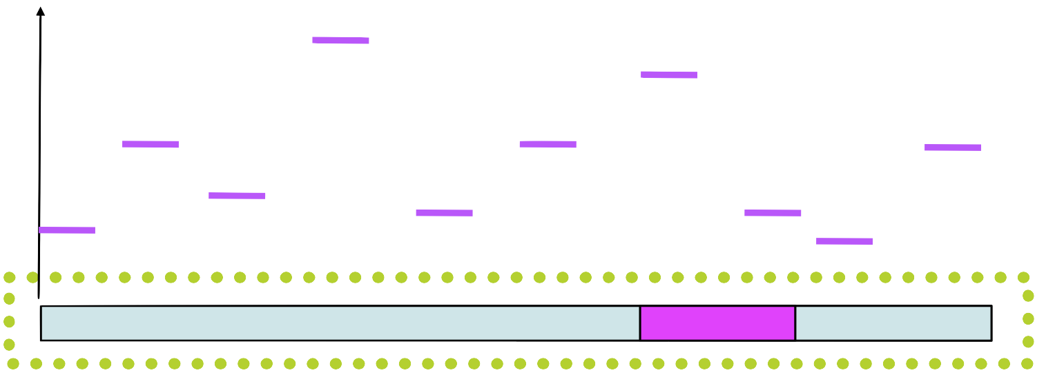
Some positions are critical, others are not
In some columns the scores can be very high
Since we know the frequency of each letter, we can calculate the average score for each column
\[\forall j \quad I(j) = \sum_X f(X, j) M(X, j)\]
It looks like this
![]()
Graphical representation of a motif
A Sequence Logo shows the frequency of each residue and the level of conservation
![]()
Why some letters are taller than others?
Application
Looking for new Binding Sites
Finding Binding Sites
Now we will look in all the genome \(G\)
For each position \(i\) in the genome, we calculate \[\text{Score}(G,i)=\sum_{j=1}^n M(G_{i+j-1}, j)\]
This will give us a vector of scores. Higher values are better
We keep all position with score higher than a threshold
The threshold depends on the statistical significance of the score
Exercise
- Go To http://meme-suite.org/
- Use MAST to find all instances of Fur motifs on S.pombe
- What are the differences between FIMO, MAST, MCAST and GLAM2Scan?
- What are the differences between MEME, DREME, MEME-ChIP, GLAM2 and MoMo?
How to find motifs
Finding new motif instances
If we know the PSSM, it is easy to find new sites matching the motif
We just use the PSSM to give a score to each symbol, and we get a total score.
High scores will be new motif instances
How to find motifs without alignment
It is easy to prepare PSSM in a multiple alignment
But we have seen that multiple alignment can be expensive
When we are looking for short patterns (a.k.a motifs) we can use other strategies
Nucleic Acids Research, Volume 34, Issue 11, 1 January 2006, Pages 3267–3278, https://doi.org/10.1093/nar/gkl429
Formalization
Given \(N\) sequences of length \(m\): \(s_1, s_2, ..., s_N\), and a fixed motif width \(k,\) we want
- a subsequence of size \(k\) (a \(k\)-mer) that is over-represented among the \(N\) sequences
- or a set of highly similar \(k\)-mers that are over-represented
Testing all sets of \(k\)-mers is computationally intensive, so several heuristics have been proposed
Gibbs Sampling Algorithm
Given \(N\) sequences of length \(m\) and desired motif width \(k\):
Step 1: Choose a position in each sequence at random: \[a_1 \in s_1, a_2 \in s_2, ..., a_N \in s_N\]
Step 2: Choose a sequence at random from the set (let’s say, \(s_j\)).
Step 3: Make a PSSM of width \(k\) from the sites in all sequences except \(s_j.\)
Gibbs Sampling Algorithm (cont)
Step 4: Assign a score to each position in \(s_j\) using the PSSM constructed in step 3: \[p_1, p_2, p_3, ..., p_{m-k+1}\]
Step 5: Choose a starting position in \(s_j\) (higher score have higher probability) and set \(a_j\) to this new position.
Gibbs Sampling Algorithm (cont)
Step 6: Choose a sequence at random from the set (say, \(s_{j'}\)).
Step 7: Make a PSSM of width \(k\) from the sites in all sequences except \(s_{j'}\), but including \(a_j\) in \(s_j\)
Step 8: Repeat until convergence (of positions or motif model)
Step 1
Choose a position \(a_i\) in each sequence at random 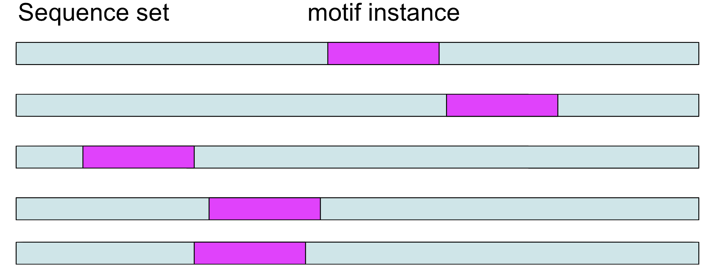
Step 2 and 3
Choose a sequence at random, let’s say \(s_1.\) Make a PSSM from the sites in all sequences except \(s_1\) 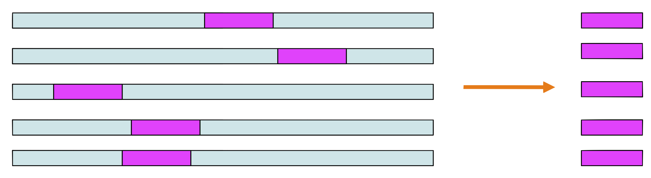
Step 4
Assign a score to each position in using the PSSM
Step 5
Choose a new position in \(s_1\) based on this score 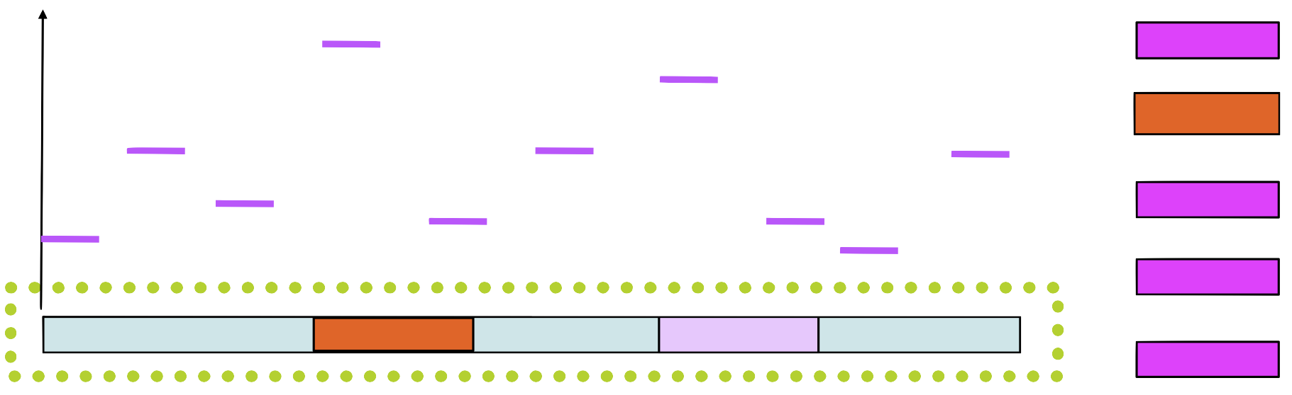
Step 6
Build a new PSSM with the new sequence 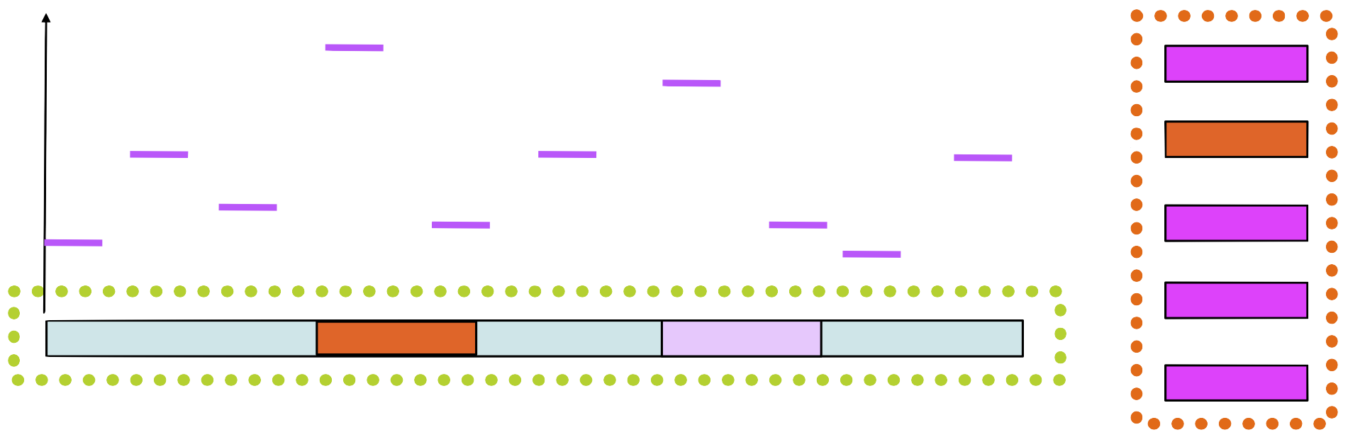
Step 7
Choose randomly a new sequence from the set and repeat 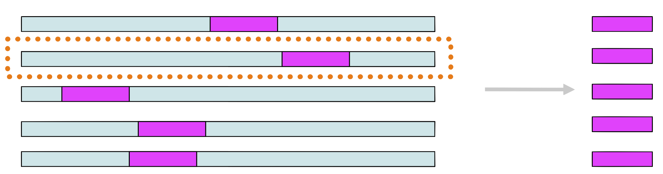
Convergence
We repeat the steps until the PSSM no longer changes
Alternative: we stop when the positions \(a_i\) do not change
The methods probably gives us a over-represented motif
Implementation
- Gibbs Motif Sampler Homepage: http://ccmbweb.ccv.brown.edu/gibbs/gibbs.html
- MotifSuite: http://bioinformatics.intec.ugent.be/MotifSuite/Index.htm
- MEME on the MEME/MAST suite