Class 6: Scoring Global and Local Alignments
Bioinformatics
Andrés Aravena
13 November 2020
In the previous class…
- Looking in databases
- Compare query against each subject in the database
- Partial match
- Find subjects with smallest distance
- Hamming distance: count mismatches
- Levenstein distance: count mismatches and indels
- Dot plots
- Global and semiglobal alignment
We showed Edit distance
“Distance” means that smaller numbers are better
If the distance is 0, then the two sequences are identical
If the distance is small, the two sequences are similar
If the distance is big, the sequences are different
Different alignments for different questions
- Global alignment compares genes to genes, or proteins to proteins
- We expect that both sequences are similar
- Semi-global alignment compares genes to genomes
- We expect that query is similar to part of subject
- Local alignment compares genomes to genomes
- We expect that part of the query is similar to part of subject
Global, Semi-Global and Local alignment
- Global
- all sequences must match.
- Each gap is penalized
- Semi-global
- all sequences must match, but one may be shorter than the other.
- external gaps are not penalized
- Local
- Some part of the sequence must match
- external gaps are not penalized
- can be with or without internal gaps
Global v/s local
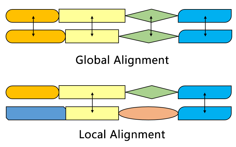
Wikipedia
Part of query to part of subject
ABRACADABRA
CHUPACABRA
Extrernal gaps do not count
      ABRACADABRA
      ||||
CHUPACABRA
Local alignment is not a distance
Since external gaps do not count, we can always use them
In this case the smallest distance is always 0
The smallest cost is achieved taking one letter
         ABRACADABRA
         |
CHUPACABRA
We cannot solve the minimization problem
Score instead of distance
Instead of finding a minimum, we look for a maximum
- Matching places get positive score
- Mismatch and gaps get negative score
The philosophy is the same, but we look for big numbers instead of small numbers
That is, we look for Optimal Alignment
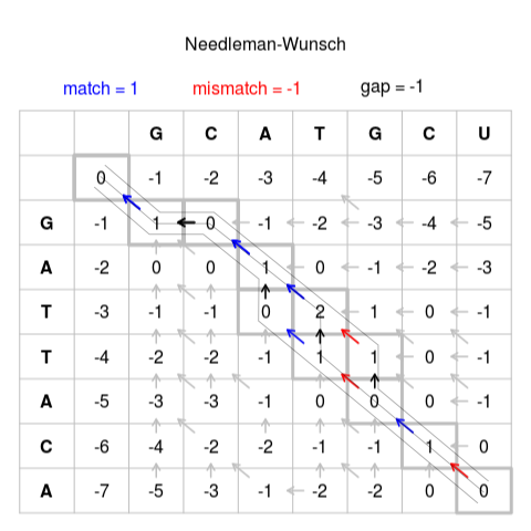
Dot plot becomes a matrix
Initially we placed 1 or 0 on each cell depending on match or mismatch
Now we put positive or negative numbers, depending of single-letter scores
We can find optimal alignment efficiently
Once the “dot plot matrix” is complete, it is easy to find the optimal score
Global alignment: find the largest sum from corner to corner
Semi-global alignment: find the largest sum from side to side
Local alignment: find the largest sum in any diagonal
BLAST
The most common tool for local alignment is BLAST
Basic Local Alignment Search Tool
BLAST is not Global Alignment
Substitution scoring matrices
Single-letter scores (example)
If we pair two letters \(x\) and \(y\), we need to know how they contribute to the score value. For example,
- If \(x = y\) the score increases by 1
- If \(x ≠ y\) the score decreases by 1
- If one of the letters is
-(a gap), the score reduces by 2
In general, we have a substitution matrix \(C_{x, y}\) for each \(x\) and \(y\)
Single-letter scores (example)
In one equation
\[C_{x, y} = \begin{cases} +1 & \quad x=y\\ -1 & \quad x≠y\\ -2 & \quad x=\texttt{"-"} \\ -2 & \quad y=\texttt{"-"} \end{cases}\]
Scoring matrices
The scoring matrix (also known as a substitution matrix) has one row and one column for each letter in our alphabet
For example 4 rows and 4 columns for DNA sequences
In DNA it is common to have +1 for match and -2 for mismatch
Sometimes we can use (+1,-3), (+1,-1) or even (4,-5)
DNA scoring matrix
   A  C  G  T
A  1 -2 -2 -2
C -2  1 -2 -2
G -2 -2  1 -2
T -2 -2 -2  1
Amino-acid scoring matrices
For proteins the alphabet has 20 letters, so the scoring matrix is 20×20
The scores of these matrices are based on the relative frequency of each mutation in nature
Obviously, we only care about non-lethal mutations
More specifically, we care about the Point Mutations that are Accepted
These are called PAM matrices (Margaret Dayhoff, 1978)
PAM matrices
Based on 1572 mutations in 71 families of closely related proteins
Dayhoff only used alignments having at least 85% identity
She assumed that any aligned mismatches were the result of a single mutation event, rather than several at the same location
PAM matrices
PAM1 is the scoring matrix for proteins in a “short” period
With some easy mathematics we can calculate PAM2, PAM30, PAM250, etc
They represent mutations in 2, 30, and 250 short periods
PAM30 matrix
    A   R   N   D   C   Q   E   G   H   I   L   K   M   F   P   S   T   W   Y   V   B   J   Z   X   *
A   6  -7  -4  -3  -6  -4  -2  -2  -7  -5  -6  -7  -5  -8  -2   0  -1 -13  -8  -2  -3  -6  -3  -1 -17
R  -7   8  -6 -10  -8  -2  -9  -9  -2  -5  -8   0  -4  -9  -4  -3  -6  -2 -10  -8  -7  -7  -4  -1 -17
N  -4  -6   8   2 -11  -3  -2  -3   0  -5  -7  -1  -9  -9  -6   0  -2  -8  -4  -8   6  -6  -3  -1 -17
D  -3 -10   2   8 -14  -2   2  -3  -4  -7 -12  -4 -11 -15  -8  -4  -5 -15 -11  -8   6 -10   1  -1 -17
C  -6  -8 -11 -14  10 -14 -14  -9  -7  -6 -15 -14 -13 -13  -8  -3  -8 -15  -4  -6 -12  -9 -14  -1 -17
Q  -4  -2  -3  -2 -14   8   1  -7   1  -8  -5  -3  -4 -13  -3  -5  -5 -13 -12  -7  -3  -5   6  -1 -17
E  -2  -9  -2   2 -14   1   8  -4  -5  -5  -9  -4  -7 -14  -5  -4  -6 -17  -8  -6   1  -7   6  -1 -17
G  -2  -9  -3  -3  -9  -7  -4   6  -9 -11 -10  -7  -8  -9  -6  -2  -6 -15 -14  -5  -3 -10  -5  -1 -17
H  -7  -2   0  -4  -7   1  -5  -9   9  -9  -6  -6 -10  -6  -4  -6  -7  -7  -3  -6  -1  -7  -1  -1 -17
I  -5  -5  -5  -7  -6  -8  -5 -11  -9   8  -1  -6  -1  -2  -8  -7  -2 -14  -6   2  -6   5  -6  -1 -17
L  -6  -8  -7 -12 -15  -5  -9 -10  -6  -1   7  -8   1  -3  -7  -8  -7  -6  -7  -2  -9   6  -7  -1 -17
K  -7   0  -1  -4 -14  -3  -4  -7  -6  -6  -8   7  -2 -14  -6  -4  -3 -12  -9  -9  -2  -7  -4  -1 -17
M  -5  -4  -9 -11 -13  -4  -7  -8 -10  -1   1  -2  11  -4  -8  -5  -4 -13 -11  -1 -10   0  -5  -1 -17
F  -8  -9  -9 -15 -13 -13 -14  -9  -6  -2  -3 -14  -4   9 -10  -6  -9  -4   2  -8 -10  -2 -13  -1 -17
P  -2  -4  -6  -8  -8  -3  -5  -6  -4  -8  -7  -6  -8 -10   8  -2  -4 -14 -13  -6  -7  -7  -4  -1 -17
S   0  -3   0  -4  -3  -5  -4  -2  -6  -7  -8  -4  -5  -6  -2   6   0  -5  -7  -6  -1  -8  -5  -1 -17
T  -1  -6  -2  -5  -8  -5  -6  -6  -7  -2  -7  -3  -4  -9  -4   0   7 -13  -6  -3  -3  -5  -6  -1 -17
W -13  -2  -8 -15 -15 -13 -17 -15  -7 -14  -6 -12 -13  -4 -14  -5 -13  13  -5 -15 -10  -7 -14  -1 -17
Y  -8 -10  -4 -11  -4 -12  -8 -14  -3  -6  -7  -9 -11   2 -13  -7  -6  -5  10  -7  -6  -7  -9  -1 -17
V  -2  -8  -8  -8  -6  -7  -6  -5  -6   2  -2  -9  -1  -8  -6  -6  -3 -15  -7   7  -8   0  -6  -1 -17
B  -3  -7   6   6 -12  -3   1  -3  -1  -6  -9  -2 -10 -10  -7  -1  -3 -10  -6  -8   6  -8   0  -1 -17
J  -6  -7  -6 -10  -9  -5  -7 -10  -7   5   6  -7   0  -2  -7  -8  -5  -7  -7   0  -8   6  -6  -1 -17
Z  -3  -4  -3   1 -14   6   6  -5  -1  -6  -7  -4  -5 -13  -4  -5  -6 -14  -9  -6   0  -6   6  -1 -17
X  -1  -1  -1  -1  -1  -1  -1  -1  -1  -1  -1  -1  -1  -1  -1  -1  -1  -1  -1  -1  -1  -1  -1  -1 -17
* -17 -17 -17 -17 -17 -17 -17 -17 -17 -17 -17 -17 -17 -17 -17 -17 -17 -17 -17 -17 -17 -17 -17 -17   1
BLOSUM matrices
Using local alignment we can identify conserved regions
In 1992 Steven Henikoff and Jorja Henikoff created new substitution matrices based on local alignment of blocks
BLOcks SUbstitution Matrix
Idea: each protein domain can evolve at different speeds
BLOSUM62
   A  R  N  D  C  Q  E  G  H  I  L  K  M  F  P  S  T  W  Y  V  B  J  Z  X  *
A  4 -1 -2 -2  0 -1 -1  0 -2 -1 -1 -1 -1 -2 -1  1  0 -3 -2  0 -2 -1 -1 -1 -4
R -1  5  0 -2 -3  1  0 -2  0 -3 -2  2 -1 -3 -2 -1 -1 -3 -2 -3 -1 -2  0 -1 -4
N -2  0  6  1 -3  0  0  0  1 -3 -3  0 -2 -3 -2  1  0 -4 -2 -3  4 -3  0 -1 -4
D -2 -2  1  6 -3  0  2 -1 -1 -3 -4 -1 -3 -3 -1  0 -1 -4 -3 -3  4 -3  1 -1 -4
C  0 -3 -3 -3  9 -3 -4 -3 -3 -1 -1 -3 -1 -2 -3 -1 -1 -2 -2 -1 -3 -1 -3 -1 -4
Q -1  1  0  0 -3  5  2 -2  0 -3 -2  1  0 -3 -1  0 -1 -2 -1 -2  0 -2  4 -1 -4
E -1  0  0  2 -4  2  5 -2  0 -3 -3  1 -2 -3 -1  0 -1 -3 -2 -2  1 -3  4 -1 -4
G  0 -2  0 -1 -3 -2 -2  6 -2 -4 -4 -2 -3 -3 -2  0 -2 -2 -3 -3 -1 -4 -2 -1 -4
H -2  0  1 -1 -3  0  0 -2  8 -3 -3 -1 -2 -1 -2 -1 -2 -2  2 -3  0 -3  0 -1 -4
I -1 -3 -3 -3 -1 -3 -3 -4 -3  4  2 -3  1  0 -3 -2 -1 -3 -1  3 -3  3 -3 -1 -4
L -1 -2 -3 -4 -1 -2 -3 -4 -3  2  4 -2  2  0 -3 -2 -1 -2 -1  1 -4  3 -3 -1 -4
K -1  2  0 -1 -3  1  1 -2 -1 -3 -2  5 -1 -3 -1  0 -1 -3 -2 -2  0 -3  1 -1 -4
M -1 -1 -2 -3 -1  0 -2 -3 -2  1  2 -1  5  0 -2 -1 -1 -1 -1  1 -3  2 -1 -1 -4
F -2 -3 -3 -3 -2 -3 -3 -3 -1  0  0 -3  0  6 -4 -2 -2  1  3 -1 -3  0 -3 -1 -4
P -1 -2 -2 -1 -3 -1 -1 -2 -2 -3 -3 -1 -2 -4  7 -1 -1 -4 -3 -2 -2 -3 -1 -1 -4
S  1 -1  1  0 -1  0  0  0 -1 -2 -2  0 -1 -2 -1  4  1 -3 -2 -2  0 -2  0 -1 -4
T  0 -1  0 -1 -1 -1 -1 -2 -2 -1 -1 -1 -1 -2 -1  1  5 -2 -2  0 -1 -1 -1 -1 -4
W -3 -3 -4 -4 -2 -2 -3 -2 -2 -3 -2 -3 -1  1 -4 -3 -2 11  2 -3 -4 -2 -2 -1 -4
Y -2 -2 -2 -3 -2 -1 -2 -3  2 -1 -1 -2 -1  3 -3 -2 -2  2  7 -1 -3 -1 -2 -1 -4
V  0 -3 -3 -3 -1 -2 -2 -3 -3  3  1 -2  1 -1 -2 -2  0 -3 -1  4 -3  2 -2 -1 -4
B -2 -1  4  4 -3  0  1 -1  0 -3 -4  0 -3 -3 -2  0 -1 -4 -3 -3  4 -3  0 -1 -4
J -1 -2 -3 -3 -1 -2 -3 -4 -3  3  3 -3  2  0 -3 -2 -1 -2 -1  2 -3  3 -3 -1 -4
Z -1  0  0  1 -3  4  4 -2  0 -3 -3  1 -1 -3 -1  0 -1 -2 -2 -2  0 -3  4 -1 -4
X -1 -1 -1 -1 -1 -1 -1 -1 -1 -1 -1 -1 -1 -1 -1 -1 -1 -1 -1 -1 -1 -1 -1 -1 -4
* -4 -4 -4 -4 -4 -4 -4 -4 -4 -4 -4 -4 -4 -4 -4 -4 -4 -4 -4 -4 -4 -4 -4 -4  1
Gaps
Gap penalty
We prefer this alignment
GGGTAACCTACCTC
||| ||||| ||||
GGGCAACCTGCCTC
instead of this other alignment
GGGT-AACCTA-CCTC
|||  |||||  ||||
GGG-CAACCT-GCCTC
Thus, gap penalty must be greater than mismatch penalty
Long gaps instead of short ones
We prefer this alignment
TCAAAGAG---GATA
|||  |||   ||||
TCA--GAGGGGGATA
instead of this other alignment
TCAAAGA-G-G-ATA
|| | || | | |||
TC-A-GAGGGGGATA
We want few long gaps instead of many short gaps
Affine gaps
Gap values must reflect how real insertions and deletions occur in nature
We observe that, once an indel event starts, it can easily grow
If the polymerase jumps, then it can jump a long distance
To represent this, we use affine gaps
Linear v/s affine
So far we considered only linear gaps
The penalty of \(n\) consecutive gaps is \(n\cdot G\)
(\(G\) is the gap penalty)
Now we consider affine gaps, where the first gap is expensive, but the consecutive are cheap
The penalty of \(n\) consecutive gaps is \(I + n\cdot E\)
\(I\) is the initial gap penalty, \(E\) is the gap extension penalty
Traceback
Traceback
After we built the matrix, we must go back from the “optimal score” finding which was the path
There may be more than one solution
Some programs build the alignment at the same time they build the matrix, but that requires more memory
Example
Solution 1
GCAT-GCU
G-ATTACA
Solution 2
GCA-TGCU
G-ATTACA
Solution 3
GCATG-CU
G-ATTACA
Alignment score depends on Substitution matrix
Score can change
If mismatches and gaps have different cost, the score will change
Sometimes the optimal alignment changes
Therefore alignments are meaningless without knowing the scoring matrices
Later we will discuss how to choose the “best” scoring matrix for each case
What is the best score?
We want big scores
How big is big enough?
We need to make several hypothesis
The most common hypothesis is statistical
Larger scores, less hits
A hit is a subject with score over a threshold
Larger score thresholds give less hits
We can estimate the number of hits in a given database, assuming randomness
That is called Expected value
Expected value as a threshold
In practice, we choose a small Expected value
(usually called E-value)
Something like 10-5 or 10-20
What we find is not random
and maybe it is biologically meaningful
E-value depends on the database
The formula for E-value depends on
- The substitution scoring matrix
- The query size
- The database size
Same alignments in different databases have different E-value
but the same score