May 10, 2019
Spanish word for Random is Azar
Things you have to know
We have three levels of knowledge
- Knowing that …
- Knowing how to …
- Understand
We need the three levels
You must know that …
- An experiment is a random process
- We don’t know the result until we do the experiment
- An experiment produces a single outcome
- Cells survival, concentration of DNA, temperature
- Outcome may be logic, factor, numeric or character
You must know that …
- Replicating the experiment produces a sample
- A sample is a vector
- Experiments produce samples, but we care about populations
You must know that …
- Populations are BIG.
- Like “all people in the planet” or “all experiments in all parallel universes”
- In the class we use known populations
- In real life populations are unknown (partially)
You must understand …
- Experiments give samples, but we care about populations
- What happens in the sample depends on the population
- By looking at the samples we can learn about the population
- Populations are big. We assume they have infinite size to make calculation easier.
You must know how to …
- Simulate experiments using the
sample()function - Prepare the
outcomesvector - Use
sample(outcomes, size=n)to getnrandom elements fromoutcomes
You must know that …
- Most times (but not always) we use
replace=TRUE - This allows
sizebigger thanlength(outcomes) - More important: probabilities do not change
You must know that …
- When population is small, sampling will change the population
- We do not do this in this course
- When population is big, sampling has a very small effect
- The difference between 1E8 and 1E8-1 is not important
- When populations have infinite size, taking a sample has no effect
- When we replace the sample, there is no effect on the population
- Sampling with replacement is the same as having an infinite population
You must understand …
- Samples are never the same, but they are similar
- Bigger sample sizes will produce more similar results
- Samples tell us something about the population
You must know that …
- The probability of an outcome is the proportion of that outcome in the population
- In real life we usually do not know the probabilities, and we want to find them
- In some cases we do know the probability of each outcome
- Then we can simulate the experiment
You must know that …
- When we use
sample, each outcome can have a different probability - The probability distribution is a vector with the same length as outcomes
- We can use the option
prob=to change the probability distribution - If we do not use
prob=, then all outcomes have the same probability
You must know how …
- Decompose a complex random process in smaller parts
- Simulate a complex random system and find the empirical frequencies
- Draw the results in a bar plot
- Use the option
prob=pto change howsample()works
You must know that …
- These simulations are called “Monte-Carlo Methods”
- This allow us to explore cases that have too many combinations
- We cannot see all possible genes of length 1000bp
- There are 41000 = 22000 = 210x200 ≈ 103x200 = 10600 combinations
- The age of the universe is ≈ 4.32x10¹⁷ seconds
You must understand …
Testing all possible cases is impossible
Random sampling allows us to get an idea of all possible cases
More simulations give better approximations, but take longer time
This is one of the most common uses of computers in Science
Events: You must know that …
- An event is any logical question about the experiment outcome, such as “two people have the same birthday”
- In R we can use functions, taking an outcome and returning
TRUEorFALSE
- In R we can use functions, taking an outcome and returning
- Outcomes and events are different
- An event can be true for several different outcomes
- An experiment produces only one outcome, and several events
Events: You must know how to …
Write a function to represent an event
- Takes a sample (one or more outcomes) as input
- Returns
TRUEorFALSEdepending on the event rule - Example:
- Two people in the course have the same birthday
- A student pass this course
You must know that …
- A random variable is any numeric value that depends on the experiment outcome, such as “the number of people with epilepsy in our course”
- In R we can use a numeric
outcomesvector
- In R we can use a numeric
- In this case there is a population average, population variance and population standard deviation
- In general we do not know the population average, and we want to know it
You must know that …
The population standard deviation measures the population width
Chebyshev theorem says \[\Pr(\vert x_i-\bar{\mathbf x}\vert\geq k\cdot\text{sd}(\mathbf x))\leq 1/k^2\] It can also be written as \[\Pr(\vert x_i-\bar{\mathbf x}\vert\leq k\cdot\text{sd}(\mathbf x))\geq 1-1/k^2\]
Chebyshev: You must know how to …
Find the population width for different values of \(k\)
- at least 75% of the population is near the average, by no more than 2 times the standard deviation \[\Pr(\vert x_i-\bar{\mathbf{x}}\vert\leq 2\cdot\text{sd}(\mathbf x))\geq 1-1/2^2\] \[\Pr(\bar{\mathbf{x}} -2\cdot\text{sd}(\mathbf x)\leq x_i \leq \bar{\mathbf{x}} +2\cdot\text{sd}(\mathbf x)) \geq 0.75\]
- at least 88.9% of the population is near the average, by less than 3 times the standard deviation \[\Pr(\bar{\mathbf{x}} -3\cdot\text{sd}(\mathbf x)\leq x_i \leq \bar{\mathbf{x}} +3\cdot\text{sd}(\mathbf x)) \geq 0.889\]
Exercise
Which value of \(k\) will give you an interval containing at least 99% of the population?
(this 99% is called confidence level)
You must understand …
Everything we measure will be in an interval
The interval depends on the population standard deviation and the confidence level
Chebyshev theorem is always true, but in some cases is pessimistic
In some cases we can have better confidence levels
You must know that …
- You can take the average of a sample to estimate the population average
- The sample average is a random variable. Changes on every experiment
- When the sample is bigger, the sample average will be closer to the population average
- This is called Law of Large Numbers
- Moreover, the sample average of a big sample will follow a Normal distribution
- This is called Central Limit Theorem
Normal distribution
 Here outcomes are real numbers
Any real number is possible
Probability of any \(x\) is zero (!)
We look for probabilities of intervals
Probabilities of Normal Distribution
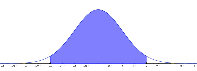
≈95% of normal population is between \(-2\cdot\text{sd}(\mathbf x)\) and \(2\cdot\text{sd}(\mathbf x)\)
≈99% of normal population is between \(-3\cdot\text{sd}(\mathbf x)\) and \(3\cdot\text{sd}(\mathbf x)\)
You must understand that ….
- The Chebyshev rule is always valid, but pessimist
- confidence intervals are big
- If the probability distribution is Normal, we can have better confidence intervals
- Not all probabilities are Normal
- When the random process is a sum of many parts, then we may have a Normal distribution
- That happens with experimental measurements
- Also happens in many biological processes
Finding Normal confidence interval
If we have 95% of population in the center, then we have 2.5% to the left and 2.5% to the right
We can find the \(k\) value using R
qnorm(0.025)
[1] -1.96
qnorm(0.975)
[1] 1.96
Finding Normal confidence interval (in general)
If we have \(1-\alpha\) of population in the center, then we have \(\alpha/2\) to the left and \(\alpha/2\) to the right
qnorm(alpha/2)
qnorm(1-alpha/2)
Now you can find any interval
The problem with confidence
You may have noticed that we never get 100% confidence
That is a fact of life. We have to accept
To have very high confidence, we need wide intervals
But wide intervals are less useful
Theory of Population Averages
Some definitions
Probability distribution
Distribution: probability of each outcome
When the outcome is numeric (i.e. when it is a random variable), the distribution is
- a vector, for discrete outcomes
- a function, for continuous outcomes (real valued random variables)
Random variable: a function of outcomes
- An experiment produces an outcome \(X\)
- For example, \(X=\) the DNA sequence of a gene
- We can calculate many numeric functions \(f(X)\) from this outcome
- For example, \(f(X)=\) length of the gene
- or \(f(X)=\) GC content of the gene
- We want to know the average of \(f(X)\) in the population
- we can only calculate averages when we have numbers
Population average of \(f(X)\)
We will represent population averages like this \[\langle f(X)\rangle \] The brackets \(\langle \quad \rangle\) represent population average
Do not confuse it with \(\bar x=\text{mean}(x)\) (sample average)
Definition of Population Average
The population is big, therefore \(N\to \infty\) and \[\frac{1}{N}\sum_{x\in\text{Population}} f(x)\quad\xrightarrow{N\to \infty}\quad \langle f(X)\rangle \] If we know the proportion of each outcome in the population, we can write \[\frac{1}{N}\sum_{x\in\text{Population}} f(x)= \sum_{a\in\text{Outcomes}} \frac{n_a}{N}f(a)= \sum_{a\in\text{Outcomes}} p_a \cdot f(a)\]
Easy case: when X is a number
If the outcomes are numbers, like optical density or concentration, then the function \(f(X)\) can be simply \[f(X)=X\] In that case the population average is simply \[\langle X\rangle\] (it’s easy, no?)
Properties of population averages
If \(X\) and \(Y\) are two random variables, then \[\langle X+Y\rangle = \langle X\rangle + \langle Y\rangle \] i.e. the average of the sum is the sum of the averages
If \(k\) is a fixed (non-random) number, then \[\langle k\, X\rangle = k\, \langle X\rangle\] i.e. constants can get out of averages
Variance
Variance is the average square error. Can be used for any function \(X\)
- error means difference between each element and the average \[X-\langle X\rangle\]
- square error means the square of the error \[(X-\langle X\rangle)^2\]
- Therefore, population average square error is \[\langle(X-\langle X\rangle)^2\rangle\]
Population Variance
We will represent population variance like this \[\mathbb V(X)=\langle(X-\langle X\rangle)^2\rangle\] Do not confuse it with sample variance \(\text{var}(x)\)
Same idea, but different context
Variance formula Shortcut
It is good to know that \[\mathbb V(X)=\langle(X-\langle X\rangle)^2\rangle=\langle X^2\rangle-\langle X\rangle^2\]
Variance is the average of squares minus the square of average
Exercise: verify that this is true
Properties of Population Variance
If \(X\) and \(Y\) are two independent random variables, then \[\mathbb V(X+Y) = \mathbb V(X) + \mathbb V(Y) \] i.e. the variance of the sum is the sum of the variances
If \(k\) is a fixed (non-random) number, then \[\mathbb V(k\, X) = k^2\, \mathbb V(X)\] i.e. the variance is multiplied by the square
Exercise: verify that this is true
Standard deviation
Variance is easy to calculate and has good properties. But the values are too big.
In practice we use the square root of variance, called standard deviation
We will represent population standard deviation like this \[\mathbb S(X)=\sqrt{\langle(X-\langle X\rangle)^2\rangle}=\sqrt{\langle X^2\rangle-\langle X\rangle^2}\] Do not confuse it with sample standard deviation \(\text{sd}(x)\)
Properties of Standard Deviation
If \(X\) and \(Y\) are two independent random variables, then \[\mathbb S(X+Y) = \sqrt{\mathbb{S}(X)^2 + \mathbb{S}(Y)^2} \] i.e. the same formula of Pythagoras’ theorem
If \(k\) is a fixed (non-random) number, then \[\mathbb S(k\, X) = k\, \mathbb S(X)\] i.e. the variance is multiplied by the square
Exercise: verify that this is true
Application 1: sums of random numbers
Imagine that we repeat the experiment \(m\) times. In other words, the sample size is \(m\)
We get the values \(x_1, x_2,\ldots, x_m.\) All result from the same experiment, with the same probabilities
We want to see what happens with \[\sum_{i=1}^m x_i\]
Application 1: sums of random numbers
Using the rules we discussed before, we have \[\left\langle\sum_{i=1}^m x_i\right\rangle=\sum_{i=1}^m \langle X\rangle=m\,\langle X\rangle\] The average of the sum is \(m\) times the average of each value.
Application 1: sums of random numbers
We also have \[\mathbb V\left(\sum_{i=1}^m x_i\right)=\sum_{i=1}^m \mathbb V( X)=m\,\mathbb V(X)\] The variance of the sum is \(m\) times the variance of each value. Finally, \[\mathbb S\left(\sum_{i=1}^m x_i\right)=\sqrt{\mathbb V\left(\sum_{i=1}^m x_i\right)}=\sqrt{m}\,\mathbb S(X)\]
We have seen this before

We have seen this before

Application 2: mean of random numbers
If now we take the average of each sample, we have \[\left\langle\frac{1}{m}\sum_{i=1}^m x_i\right\rangle=\sum_{i=1}^m \frac{1}{m}\langle X\rangle=\langle X\rangle\] The population average of the sample means is the population average of each value.
Application 2: mean of random numbers
We also have \[\mathbb V\left(\frac{1}{m}\sum_{i=1}^m x_i\right)=\sum_{i=1}^m \frac{1}{m^2}\mathbb V( X)=\frac{1}{m}\mathbb V(X)\] The variance of the sample means is \(1/m\) times the variance of each value.
Application 2: mean of random numbers
Finally, \[\mathbb S\left(\frac{1}{m}\sum_{i=1}^m x_i\right)=\sqrt{\frac{1}{m}\mathbb V\left(\sum_{i=1}^m x_i\right)}=\frac{\mathbb S(X)}{\sqrt{m}}\]
We have seen this before

We have seen this before

Chebyshev theorem
If we know the average and standard deviation of population, we can say that
- at least 75% of the population are close to the average, by less than 2 times the standard deviation \[\Pr\left(\vert \bar X_m-\langle X\rangle\vert\leq 2\frac{\mathbb S(X)}{\sqrt{m}}\right)\geq 1-1/2^2\] \[\Pr\left(\langle X\rangle -2\frac{\mathbb S(X)}{\sqrt{m}}\leq \bar X_m \leq \langle X\rangle +2\frac{\mathbb S(X)}{\sqrt{m}}\right) \geq 0.75\]
Chebyshev theorem
- At least 88.9% of the population are close to the average, by less than 3 times the standard deviation \[\Pr\left(\langle X\rangle -3\frac{\mathbb S(X)}{\sqrt{m}}\leq \bar X_m \leq \langle X\rangle +3\frac{\mathbb S(X)}{\sqrt{m}}\right) \geq 0.889\]
Application 3: Central limit theorem
If we take averages from many samples, the sample average will follow a Normal distribution
Normal distribution
- 95% of the sample averages are close to the population average, at less than 2 times the standard deviation \[\Pr\left(\vert \bar X_m-\langle X\rangle\vert\leq 2\frac{\mathbb S(X)}{\sqrt{m}}\right)\approx 0.95\] \[\Pr\left(\langle X\rangle -2\frac{\mathbb S(X)}{\sqrt{m}}\leq \bar X_m \leq \langle X\rangle +2\frac{\mathbb S(X)}{\sqrt{m}}\right) \approx 0.95\]
- 99% of the sample averages are close to the population average, at less than 3 times the standard deviation \[\Pr\left(\langle X\rangle -3\frac{\mathbb S(X)}{\sqrt{m}}\leq \bar X_m \leq \langle X\rangle +3\frac{\mathbb S(X)}{\sqrt{m}}\right) \approx 0.99\]
So we can locate the population average
- 95% of the sample averages are close to the population average, at less than 2 times the standard deviation \[\Pr\left(\vert \bar X_m-\langle X\rangle\vert\leq 2\frac{\mathbb S(X)}{\sqrt{m}}\right)\approx 0.95\] \[\Pr\left(\bar X_m -2\frac{\mathbb S(X)}{\sqrt{m}}\leq \langle X\rangle\leq \bar X_m +2\frac{\mathbb S(X)}{\sqrt{m}}\right) \approx 0.95\]
So we can locate the population average
- 99% of the sample averages are close to the population average, at less than 3 times the standard deviation \[\Pr\left(\bar X_m -3\frac{\mathbb S(X)}{\sqrt{m}}\leq \langle X\rangle \leq \bar X_m+3\frac{\mathbb S(X)}{\sqrt{m}}\right) \approx 0.99\]
Confidence intervals
Bad news
We do not know the population variance
All we said before is true, but cannot be used directly
Because we do not know the population variance
Thus, we also ignore the population standard deviation
What can we do instead?
Using sample variance instead of population variance
The solution is to use the standard deviation of the sample
(do not confuse it with standard deviation of the sample means)
But we have to pay a price: lower confidence
Student’s distribution
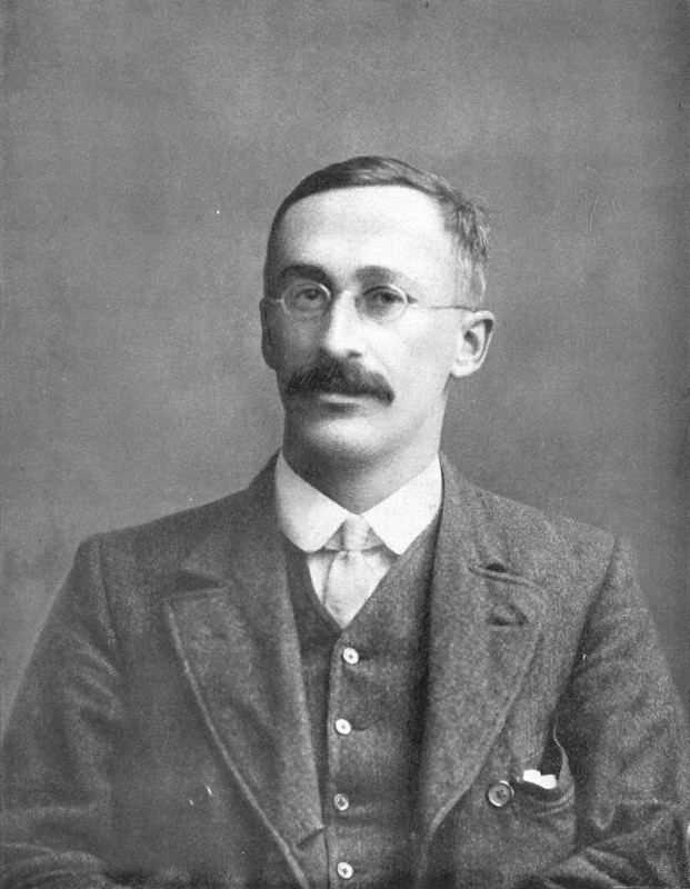
Published by William Sealy Gosset in Biometrika (1908)
He worked at the Guinness Brewery in Ireland
Studied small samples (the chemical properties of barley)
He called it “frequency distribution of standard deviations of samples drawn from a normal population”
Story says that Guinness did not want their competitors to know this quality control, so he used the pseudonym “Student”
Student’s distribution is wider than Normal
plot(x,dnorm(x), type="l", lty=2)
lines(x, dt(x, df=3), lty=1)
legend("topleft", legend = c("t-Student","Normal"), lty=1:2)

How to know the t-Student values
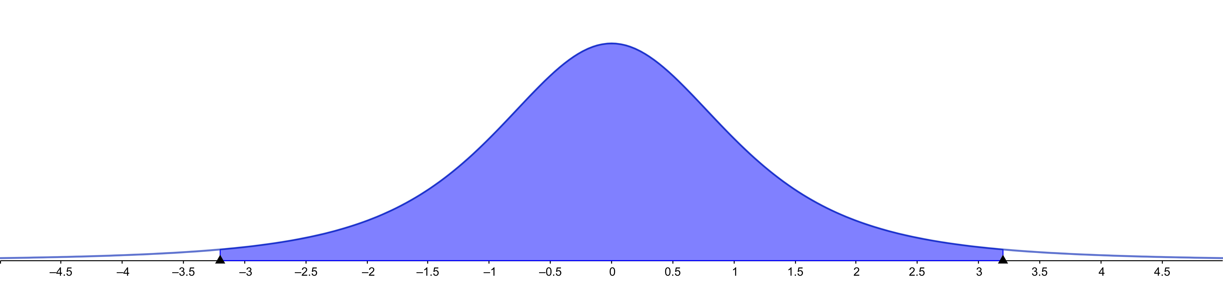
Intervals are wider (but less than with Chebyshev)
It is a family of Student’s distributions
Here we use the sample standard deviation to approximate the population standard deviation
As we have seen, if the sample is small, these two values may be different
Thus, the Student’s distribution depends on the sample size
Degrees of Freedom
The key idea is that the sample has \(m\) elements, but they are constrained by 1 value: the sample average
We say that we have \(m-1\) degrees of freedom
Degrees of Freedom

Finding Student’s confidence intervals
If we have 95% of population in the center, then we have 2.5% to the left and 2.5% to the right
We can find the \(k\) value if the sample size is 5
qt(0.025, df=5-1)
[1] -2.78
qt(0.975, df=5-1)
[1] 2.78
\(k\) depends on sample size

Summary
- Normal distributions are common in nature
- They happen when many things add together
- If the process is Normal, then the sample average is close to the population average
- The confidence interval uses the t-Student distribution