April 26, 2019
Easy and Hard problems
Life is hard, sometimes
We can say that there are two kinds of problems
- Easy problems
- Hard problems
Easy problems
… can be solved quickly
For example
5 × 7?
Hard problems
Take longer time to solve
For example
78 / 6
Solutions are easily to verify
We think that
78 / 6 = 13
We can verify this solution doing
13 × 6 = 78
Forward and Backward
It is useful to say that
- Easy problems move Forward
- Hard problems move Backward
For example
- Multiplication moves forward,
- Division moves backward,
- Verification is forward again
Easy problem
Find the value of
162
Hard problem
Find the value of
\(\sqrt{324}\)
When you find a solution, it is easy to verify
Easy problem
Multiply two prime numbers
4391 * 6113
[1] 26842183
Hard problem
Find the two prime numbers that are factors of this
[1] 26164559
All Internet security is based on this idea
Breaking Internet security is hard
It is based on factorization on prime numbers
1 Hard problem = Many Easy problems
As you can realize, if you know how to solve the forward problem, you can solve the backward problem by brute force
You try several starting points, apply the forward method and see if you find the backward end point
For example, to solve 78/6 you can try
(1:15) * 6
[1] 6 12 18 24 30 36 42 48 54 60 66 72 78 84 90
Is there a shortcut?
Is there a way that a hard problem becomes a easy problem?
In some cases, yes
In general, probably no
Nobody knows for sure. So one day Internet security may finish
If you want to know more, google “P versus NP problem”
Easy and Hard problems in Deterministic Systems
We saw this last class and in the Midterm Exam
- Easy problem: Simulate for some rates and initial conditions
- Hard problem: Find the rates or initial conditions that match a given result
For example:
- find reaction rates in a chemical reaction
- find initial DNA concentration in Real-Time qPCR
- find primer’s efficiency in PCR. That is, melting temperature, and binding energy
Easy and Hard Probability problems
Like in deterministic systems, we have two cases:
- Easy problem: if we know the probabilities we can simulate several experiments
- Hard problem: if we know the experiment results, find what are the probabilities
Probabilities
Key concepts
- Experiment
- system that produces a result. We do not know the result before
- Example: survey, dice, counting cells, a plant did grow or not, measuring cytotoxicity.
- Outcome
- result of an experiment. Only one outcome for each experiment.
- Population
- Set of all possible outcomes. Very big, we assume infinite size.
- Sample
- Set of outcomes from a few experiments. Much smaller than the population.
Population
Population is a very very big set of things
- All people in Turkey
- All humans living today
- All humans that ever lived
- All living organisms in the past and in the future
- All the infinite possible results of an experiment
You can assume that population size is infinite
All experiments’ results are also a population
We can do and redo an experiment for ever
(we just need a lot of money and grandchildren)
We can throw a dice 🎲 forever
All the (infinite) possible results are a population
The things in the population are outcomes
For example
⚀ ⚁ ⚂ ⚃ ⚄ ⚅
A, C, G, T
Experiments produce Samples
Each experiment gives us an outcome
Several experiments are a sample
They are randomly taken from the population
A Sample is a small part of population, chosen randomly
- small number of elements
- changes every time
- if we take two samples they will be different
Sampling in R
Sampling is shuffling
sample(LETTERS)
 [1] "H" "T" "J" "U" "W" "A" "K" "Q" "X" "Z" "P" "G"
[13] "R" "S" "B" "N" "C" "V" "Y" "O" "F" "D" "M" "E"
[25] "L" "I"
We can ask for the first N results
sample(LETTERS, size=5)
[1] "O" "Z" "G" "D" "V"
What are the chances?
All letters have the same chance of being the first one chosen
sample(LETTERS, size=5)
[1] "X" "R" "T" "A" "K"
But the first letter cannot be the second, o 3rd, 4th, 5th.
Every time we get an outcome, the chances change
Bigger groups
In real life, we usually sample from huge sets
- We survey some people from a city, country or planet
- We test some plants among the billions of plants
- We do some experiments among the trillions of possible experiments
In practice, our sample is small compared to the total
Therefore the effect is small and chances do not change
Chances should not change
If the population is big and our sample is small, then chances will not change
We can simulate that using a big population (bad idea)
sample(rep(LETTERS, 1e6), size=5)
Don’t do this: It takes too much time and memory.
They change very little, and we can assume they do not change
Take 5 letters with fixed chances
A possible solution is this:
ans <- rep(NA, 5)
for(i in 1:5) {
    ans[i] <- sample(LETTERS, size=1)
}
Taking one letter each time does not change the chances
Sampling with replacement
Other way of sampling without changing the chances is this
sample(LETTERS, size=5, replace=TRUE)
In this case we replace (put back) each letter we get
replace=TRUE means chances do not change
Outcomes can be anything that we can write in R
- Nucleotides
sample(c("A","C","G","T"), size, replace=TRUE)
- Amino-acids:
sample(seqinr::a(), size, replace=TRUE)`
- Alleles:
sample(c("AA","Aa","aa"), size, replace=TRUE)`
- numbers
sample(1:100, size, replace=TRUE)
Probabilities
Each random system may have some preferred outcomes
All outcomes are possible, but some can be probable
The probabilities are on what we know about the system
How to find the probabilities?
Symmetric systems
In some systems all outcomes are equivalent
There is no reason to prefer any letter to another
This is right when we have symmetry
A coin is symmetric. Each side has the same chance
A dice is symmetric. Each face has the same chance
Symmetric probabilities
When the system is symmetric, the probabilities are easy
- There are
Npossible outcomes, - They are symmetrical
- There is no reason to prefer one outcome to the other
- Therefore each probability must be
1/N
Asymmetry
In other cases different outcomes may have different proportions
For example
(A, C, C, G, G, T)
(A, A, C, C, C, G, G, G, T)
The proportions are the probabilities
In (A, C, C, G, G, T) the proportions are
- P(A)=1/6,
- P(C)=1/3,
- P(G)=1/3,
- P(T)=1/6
What about (A, A, C, C, C, G, G, G, T)?
If we know the proportion of each outcome in the population, we know its probability
Simulating an asymmetric system
If we know the probabilities, we can tell R to use them to simulate
To simulate (A, C, C, G, G, T) we use
sample(c("A","C","G","T"), size=N, replace=TRUE,
        prob=c(1/6, 1/3, 1/3, 1/6))
Two dice
For example, when we throw two dice and count points, we have
- zero ways of getting 1,
- one way of getting 2,
- six ways of getting 7,
- one way of getting 12,
- etc.
The technique for finding these numbers is called combinatorics
We will not do combinatorics here
Simulating two dice
To simulate two dice, we have
sample(1:12, size=N, replace=TRUE,
        prob=c(0,1,2,3,4,5,6,5,4,3,2,1)/36)
How do we find the probabilities
There are two different ways of figuring out probabilities
- We can use the brain, pen and paper
- That is, we can do math
- We can use our hands, laboratories and computers
- That is, we can do experiments
In this course we will do (mostly) the second way
Complex random systems
Decomposition again
If the system we want to simulate is complex, we usually do not know the probabilities
In that case we can decompose the random system
- small parts are easier to simulate
- combine them to make the complex system
Let’s experiment with two dice 🎲 🎲
We roll two dice. What is the sum 🎲 +🎲 ?
roll2 <- function() {
    dice <- sample(1:6, size=2, replace=TRUE)
    return(sum(dice))
}
roll2()
[1] 7
The output is a random outcome
Try it. What is your result?
We need to do more experiments
One experiment is meaningless
We need to replicate the experiment
ans <- rep(NA, 15)
for(i in 1:15) {
    ans[i] <- roll2()
}
Replicating
We can use the function replicate(n, expression)
replicate(15, roll2() )
[1] 4 4 6 2 5 8 4 6 6 6 9 5 5 8 10
Let’s do 200 experiments
deney <- replicate(200, roll2() )
deney
  [1]  8  9  6  5  7  4  7  8  4 12  8  5  7  4  6  7
 [17]  6  9  9 10  4  8  7  6 10  7  6  4  9  2  6 10
 [33] 10  8 10  9  5  3  8  3  7  9  5  4  6  5  7  7
 [49]  7  7  5  6 11  9  7 10  8  7  7  6 12  4 10  9
 [65]  7  5  8  8  9  5  4  5  7  6  6 11  8 10  4  7
 [81] 11  7  5  5  7  6  8  6  7  9 11  4  6  9  5  9
 [97] 12 11  8  6  5  7  2 10  9  5  6  5  4  3  6  3
[113]  7 10  7  6  6 10  7  2  6  6  6  8  8  9  8  6
[129]  2  7  9  6 11  5  9 10  4  6  6  9  6  7  5 10
[145]  8  8  3  8  8  3  6  6  9 10  7  8  9  8 10  4
[161]  3  8 10  3  3  7  7 10  6  6  8  7  5  4  8  4
[177]  8  6 10  5  7 10  8  6  4  2  6  6 11  6  8  7
[193]  3  8 10  2  9  4  6  7
We can calculate the frequency
table(deney)
deney
 2  3  4  5  6  7  8  9 10 11 12
 6 10 17 19 37 33 28 20 20  7  3
We can even make a plot
barplot(table(deney))

Absolute frequency
- Absolute frequency is how many times we see each value
- The sum of all absolute frequencies is the Number of cases
- Here the number of cases is 200
Increasing the number of cases
deney <- replicate(1000, roll2() )
barplot(table(deney))
 All numbers increase
Relative frequency
- Relative frequency is the proportion of each value in the total
- The sum of all relative frequencies is always 1 \[\text{Relative frequency} = \frac{\text{Absolute frequency}}{\text{Number of cases}}\]
Plotting relative frequencies, N=200
deney <- replicate(200, roll2() )
barplot(table(deney) / 200)

Plotting relative frequencies, N=1000
deney <- replicate(1000, roll2() )
barplot(table(deney) / 1000)

Plotting relative frequencies, N=40000
deney <- replicate(40000, roll2() )
barplot(table(deney) / 40000)

Empirical Frequencies are close to Probabilities
The result of our experiments give us empirical frequencies
They are close to the theoretical probabilities
When size is bigger, the empirical frequencies are closer and closer to the real probabilities
We know for sure that when size grows we will get the probabilities
But size has to be really big
We are absolutely sure about this
How can be really sure that when size grows we will get the probabilities?
How do we know?
We know because people has proven a Theorem
It is called Law of Large Numbers
Theorems are Eternal Truth
Mathematics is not really about numbers
Mathematics is about theorems
Finding the logical consequences of what we know
But it is all in our mind
Experiments give Nature without Truth
Math gives Truth without Nature
Science gives Truth about Nature
Samples are connected to populations
The main consequence of the Law of Large Numbers is
Samples tell us something about populations
Therefore we can learn about populations if we do experiments
In our course experiment means sample(x, size, replace=TRUE)
But we cannot see all the population
Normally it is easy to know the possible outcomes
Normally it is hard to know the probabilities
Knowing the probabilities is knowing the population
Probabilities describe what we know about the population
What is the absolute frequency of roll2()==7
freq <- table(deney)
freq["7"]
   7
6613
This is a little tricky
It is easy to make a mistake here
Notice that freq["7"] is not freq[7]
Remember that we can use text and numbers as indices.
Here freq is
freq
deney
   2    3    4    5    6    7    8    9   10   11   12
1093 2210 3411 4490 5659 6613 5577 4427 3257 2147 1116
What is freq[12]? Be careful
A safer way to get absolute frequency
If we want to know how may times we rolled a 7, we can do
sum(deney == 7)
[1] 6613
Remember that:
- Comparisons produce logic vectors
sum()of a logic vector is the number ofTRUE
What is the absolute frequency of roll2()==1
Here we are in more trouble, since there is no freq["1"]
freq["1"]
<NA>
  NA
It is better to ask in a safe way
sum(deney == 1)
[1] 0
Rolling more dice every time
It is easy to have more dice
roll_dice <- function(M) {
    dice <- sample(1:6, size=M, replace=TRUE)
    return(sum(dice))
}
The output is a random outcome
Combining outcomes
We can combine several outcomes in a logic question
An event is any logic question about an outcome
deney == 7deney > 9deneyis even
Random Variables
We can calculate values that depend on the outcome
A random variable is a function that depends on the outcome
For example, the proportion of times that an event is true
event is a logic vector. sum(event) is a number between 0 and length(event)
sum(event)/length(event)
Example: gene GC content
What is the GC content of a random gene?
You can see that GC content is a random variable
gene <- sample(c("A","C","T","G"), size,
                replace=TRUE)
gc_gene <- sum(gene=="C" | gene=="G")/length(gene)
size is the gene size. Symbol | means or
The outcome is the gene. The random variable is gc_gene
Simulate GC content
gc_one_gene <- function(M) {
    gene <- sample(c("A","C","T","G"), size=M, replace=TRUE)
    gc_gene <- sum(gene=="C" | gene=="G")/length(gene)
    return(gc_gene)
}
gc_genes <- replicate(10000, gc_one_gene(900))
Histogram of absolute frequencies
hist(gc_genes, col = "grey")

Histogram of relative frequencies
hist(gc_genes, col = "grey", freq=FALSE)

Better GC content
We can have a better simulation if we use the real proportions for ("A","C","T","G")
Let’s evaluate them for Carsonella rudii
library(seqinr)
genome <- read.fasta("AP009180.fna")
table(genome[[1]])
         a          c          g          t
0.41797046 0.08455988 0.08108379 0.41638587
Simulate again
gc_one_gene <- function(M, prob) {
    gene <- sample(c("A","C","G","T"), size=M, prob=prob,
                replace=TRUE)
    gc_gene <- sum(gene=="C" | gene=="G")/length(gene)
    return(gc_gene)
}
gc_genes <- replicate(10000, gc_one_gene(900, prob))
Histogram with corrected probabilities
hist(gc_genes, col = "grey", freq=FALSE)

Real GC content
genes <- read.fasta("c_rudii.fna.txt")
crudii_genes <- rep(NA, length(genes))
for(i in 1:length(genes)) {
  crudii_genes[i] <- GC(genes[[i]])
}
hist(crudii_genes, col="grey", freq=FALSE)

Range of GC content depends on gene size
small_genes <- replicate(10000, gc_one_gene(200, prob))
medium_genes <- replicate(10000, gc_one_gene(600, prob))
big_genes <- replicate(10000, gc_one_gene(1200, prob))

Another view of GC content v/s size

Is there any atypical gene?
Now we can estimate the probability of the GC content of each gene
We know that the probability of GC content depends on the gene size
How would you test if the GC content of a gene has low probability?
What other Random Variables can you imagine?
- Average
- Number of trials until success
- Number plants that grow in the lab
- Number of people that answer the homework
- Number of people that passes the course
What other random variable do you see?
How many times until success?
How many times will you do this course?
Depending on how many questions you ask and how many homework you do, you will have different chances of passing this course
To be neutral, let’s try with different probabilities
How many times do you need to do this course until you pass?
Counting until success
Assuming we have a function called fail(), that returns TRUE when the experiment fails; then this code gives us number of trials until sucess
k <- 1
while(fail()) {
    k <- k+1
}
Success & Failure: two sides of a coin
A simple way to model fail() is to use a coin
fail <- function() {
    coin <- sample(c("H","T"), size=1)
    return(coin != "H")
}
The symbol != means not equal
A biased coin
It will be useful to assume that heads and tails have different probabilities
You can imagine a deck of cards with cards of two colors in different proportion
Since the sum of probabilities for all outcomes is 1, and there are two possible outcomes, then
\[\Pr(\text{Tails}) = 1- \Pr(\text{Heads})\]
Simulating a biased coin
This function takes one input: the probability of success
fail <- function(p) {
    coin <- sample(c("H","T"), size=1, prob=c(p, 1-p))
    return(coin != "H")
}
Tossing a coin until Heads
roll_until_head <- function(p) {
    i<-1
    while(sample(c("H","T"), size=1,
            prob=c(p, 1-p)) != "H") {
        i <- i+1
    }
    return(i)
}
Results for 50%
sim <- replicate(1000, roll_until_head(0.5))
barplot(table(sim)/1000)

Results for 90%
sim <- replicate(1000, roll_until_head(0.9))
barplot(table(sim)/1000)

Results for 10%
sim <- replicate(1000, roll_until_head(0.1))
barplot(table(sim)/1000)

Homework
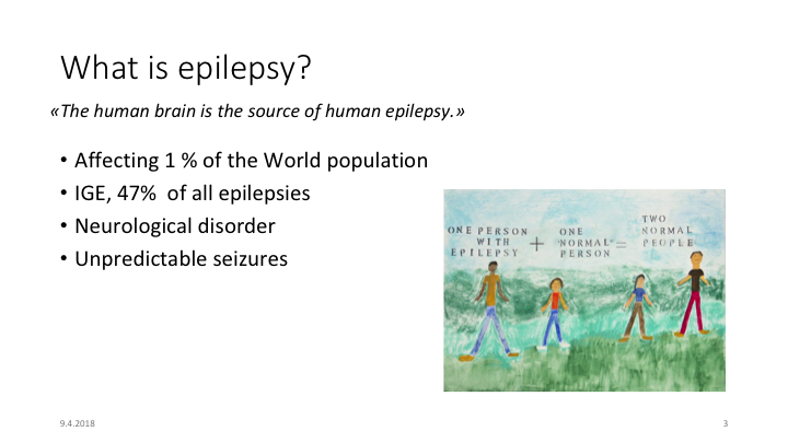
How many persons with epilepsy in our course?
Worldwide proportion is 1%
And world is a population
We are 99 people in this course, including me
Can we have 5 people with epilepsy in our class?
Birthday
What are the chances that two people have the same birthday in our class?