
March 15, 2019
Are you ready?
What do you need to know?
- Computational Thinking
- Decomposition
- Pattern Recognition
- Abstraction
- Algorithm Design
- Not about memory
- About Problem solving
Key ideas
- Loops:
for(){},while(){} - Conditional:
if(){},if(){} else {} - Recursive functions:
fac(N) = N * fac(N-1)
Practical tools
- Turtle graphics
- Normal graphics:
plot(),segments() - Reading DNA sequences
read.fasta()
DNA has two strands
FASTA files show only one strand
We call it the forward strand
The other strand is not shown, but can be calculated
We call it the reverse strand
Calculating the reverse strand
According to Watson & Crick, the reverse strand is complementary
- Change
abytand vice-versa - Change
cbygand vice-versa
Moreover, the reverse strand is reversed
- 5’ becomes 3’ and vice-versa
- i.e. we have to read it backwards
opposite_strand <- function(dna) {
    for(i in 1:length(dna)) {
        j <- length(dna) - i + 1
        if(dna[j]=='a') {
            ans[i] <- 't'
        } else if(dna[j]=='c') {
            ans[i] <- 'g'
        } else if(dna[j]=='g') {
            ans[i] <- 'c'
        } else if(dna[j]=='t') {
            ans[i] <- 'a'
        }
    }
    return(ans)
}
Warning
There is something wrong here
This code produces an error
opposite_strand(dna)
Error in opposite_strand(dna): object 'dna' not found
We can use the debugger to see what is happening
Create a vector before using it
We cannot use ans[i] if the vector ans does not exist
It has to be created before
We can create ans as a vector of NA values
ans <- rep(NA, size)
We have the new vector, but we don’t know yet the values
We need to know the vector’s size
We can create ans with this command
ans <- rep(NA, size)
For this, we need to know the size of the new vector
In this case it must be the same size as the dna vector
(because opposite strands have the same length)
opposite_strand <- function(dna) {
    ans <- rep(NA, length(dna))
    for(i in 1:length(dna)) {
        j <- length(dna) - i + 1
        if(dna[j]=='a') {
            ans[i] <- 't'
        } else if(dna[j]=='c') {
            ans[i] <- 'g'
        } else if(dna[j]=='g') {
            ans[i] <- 'c'
        } else if(dna[j]=='t') {
            ans[i] <- 'a'
        }
    }
    return(ans)
}
This is the correct version
Result
dna <-c('t','a','a','c','g','t')
dna
[1] "t" "a" "a" "c" "g" "t"
opposite_strand(dna)
[1] "a" "c" "g" "t" "t" "a"
More DNA statistics
What happens if we use the reverse strand
Will GC content change?
Will GC skew change?
Chargaff’s rules
Discovered by Austrian chemist Erwin Chargaff in 1952
DNA from any cell of all organisms has a 1:1 ratio of pyrimidine and purine bases
The amount of guanine is equal to cytosine and the amount of adenine is equal to thymine.
Chargaff E, Lipshitz R, Green C (1952). Composition of the deoxypentose nucleic acids of four genera of sea-urchin. J Biol Chem 195 (1): 155–160
Rudner, R; Karkas, JD; Chargaff, E (1968). Separation of B. Subtilis DNA into complementary strands. 3. Direct analysis. PNAS. 60 (3): 921–2.
First Chargaff’s parity rule
A double-stranded DNA molecule globally has
- %A = %T
- %G = %C
Question
Why this rule is always valid?
Second Chargaff’s parity rule
A single-stranded DNA molecule globally has
- %A ≈ %T
- %G ≈ %C
This is valid globaly for each one of the two DNA strands
If we look into small local parts of the genome then this may not be true
DNA replication
There is a richness of G over C and T over A in the leading strand
(and vice versa for the lagging strand)
GC skew changes sign at the boundaries of the two replichores
This corresponds to DNA replication origin or terminus
DNA replication
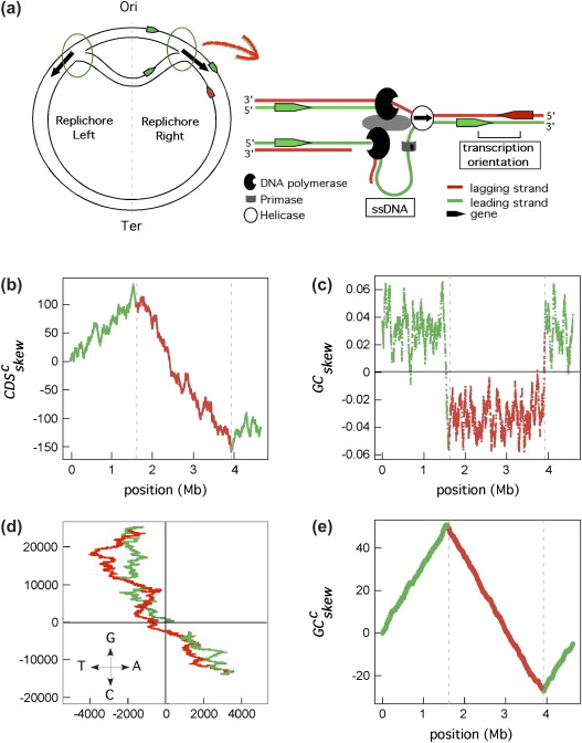
Marie Touchon, Eduardo P.C. Rocha, (2008), From GC skews to wavelets: A gentle guide to the analysis of compositional asymmetries in genomic data,
Biochimie, Volume 90, Issue 4,
Video
Finding replication origin using GC skew
The relation between %G and %C is not constant over all the genome
In some parts of the genome there are more G than C
We can evaluate this using the GC skew \[\frac{G-C}{G+C}\]
Calculating GC skew
nG <- sum(dna=="g")
nC <- sum(dna=="c")
ans <- (nG-nC)/(nG+nC)
What happens if nG+nC==0?
What to do if there are no G or C
When we examine a small part of the genome, it can happen that there are no G or C. Then, the previous program fails
This version will work better
nG <- sum(dna=="g")
nC <- sum(dna=="c")
if( (nG+nC) == 0) {
  ans <- 0
} else {
  ans <- (nG-nC)/(nG+nC)
}
Statistics in parts of the genome
Local statistics look only through a small window
A Window is a part of the genome, from an initial position, and with a fixed size
For example, we can analyze a region of 500 bp starting at position 3000 of the genome
Looking at the window
position 3000, size 500
window <- dna[3000:3499]
In the general case, we can write
window <- dna[start:(start+size-1)]
Another way to look at the window
Remember the function seq() for numeric sequences
window <- dna[seq(from=3000, length.out=500)]
In the general case, we can write
window <- dna[seq(from=start, length.out=size)]
Remember the seq() function
seq(from, to, by, length.out)
All inputs are optional
Choose carefully which ones to use
Examples of seq()
seq(from=5, to=14)
[1] 5 6 7 8 9 10 11 12 13 14
seq(from=5, length.out=10)
[1] 5 6 7 8 9 10 11 12 13 14
seq(from=5, to=30, by=3)
[1] 5 8 11 14 17 20 23 26 29
GC skew function
gc_skew <- function(dna, start, size) {
  window <- dna[seq(from=start, length.out=size)]
  nG <- sum(window=="g")
  nC <- sum(window=="c")
  if( (nG+nC) == 0) {
      return(0)
  } else {
      return( (nG-nC)/(nG+nC) )
  }
}
Sometimes DNA is in UPPER CASE
gc_skew <- function(dna, start, size) {
  window <- dna[seq(from=start, length.out=size)]
  nG <- sum(window=="g" | window=="G")
  nC <- sum(window=="c" | window=="C")
  if( (nG+nC) == 0) {
      return(0)
  } else {
      return( (nG-nC)/(nG+nC) )
  }
}
Evaluate gc_skew() on different parts of the genome
We traverse the genome with several windows of fixed size
Each window starts after the end of the previous one
In other words, the windows do not overlap
Create a vector with the window’s positions
We start at the first DNA position, until the last
Be careful to not step out of DNA
win_pos <- seq(from=1, to=length(dna)-size, by=size)
Now we apply gc_skew() to each element of win_pos
Complete code to evaluate local GC skew
For example, for windows of size 100000
size <- 1E5
win_pos <- seq(from=1, to=length(dna)-size, by=size)
skew <- rep(NA, length(win_pos))
for(i  in 1:length(win_pos)) {
    skew[i] <- gc_skew(dna, win_pos[i], size)
}
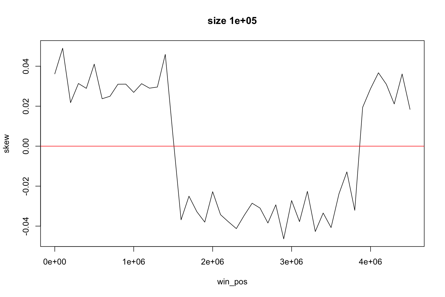
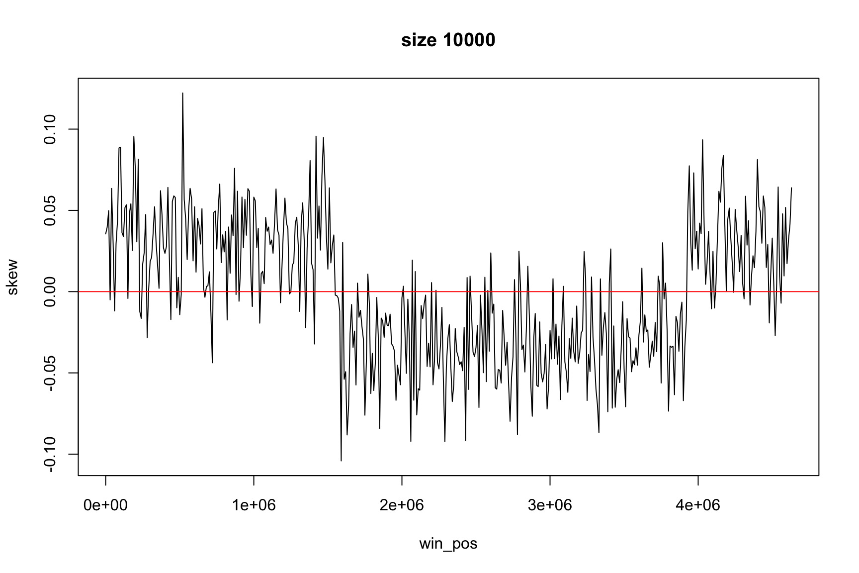
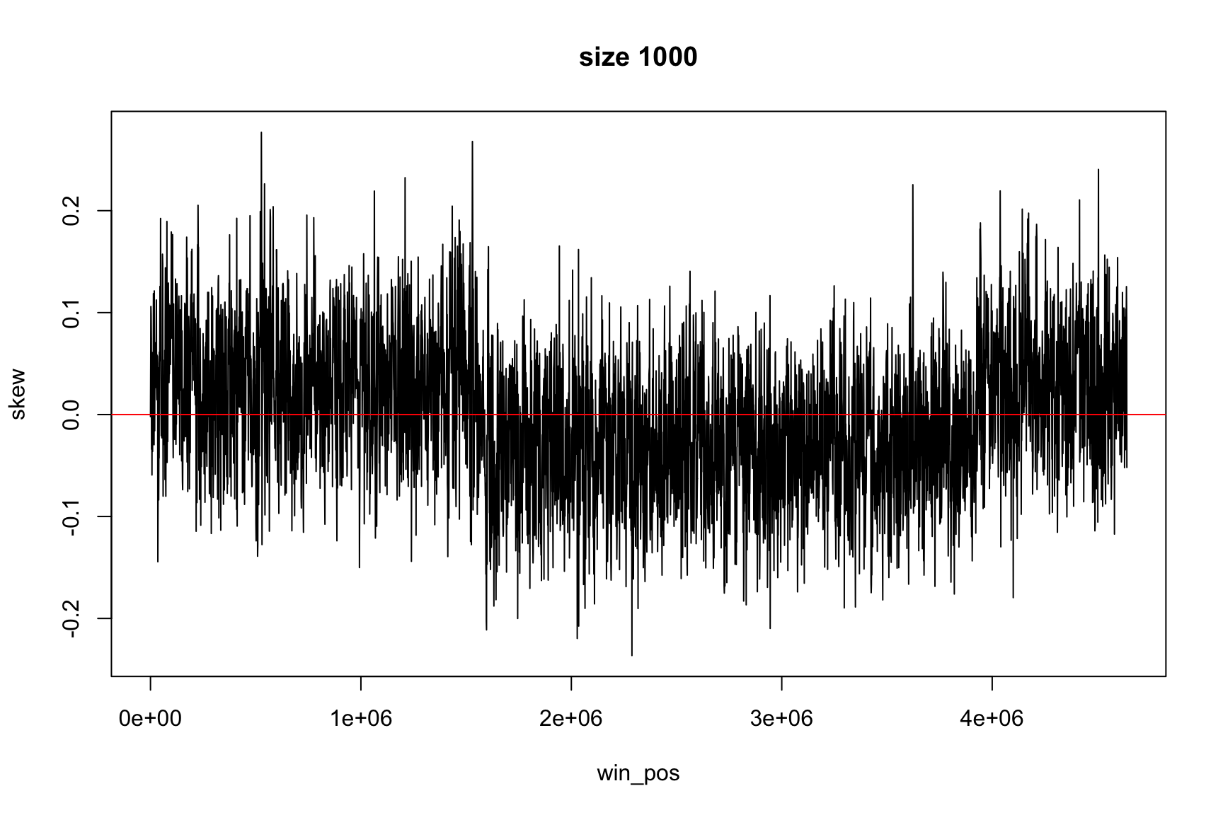
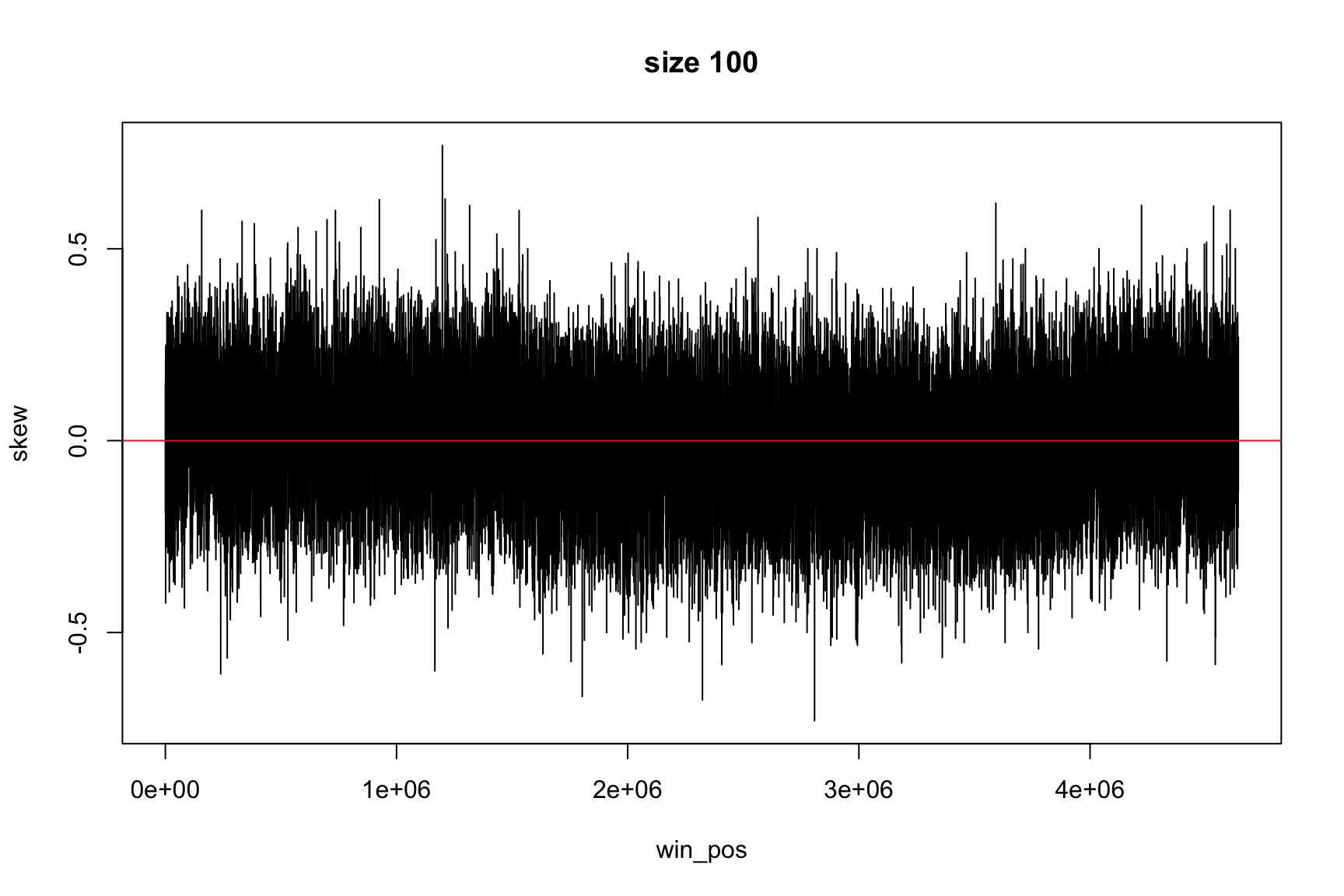
The result depends on window’s size
Result for size=1E5
Result for size=1E4
Result for size=1E3
Result for size=1E2
Finding the origin
- the GC skew is positive in one part of chromosome
- and negative on the other, on average
- it changes sign in two places
The reason for this asymmetry is the DNA replication process
The origin of replication is in one of the sign changing places
How can we find the change of sign
We want to write a program so we can find Ori on many different genomes
We can answer questions like:
- Are both replichores of the same size?
- If they are different, what is the biological reason?
- Is there some insertion?
- What are the extra genes? What do they do?
Finding the change of sign is not so easy
The values can change a lot between a window and the next one
skew data is noisy. A lot of small random changes
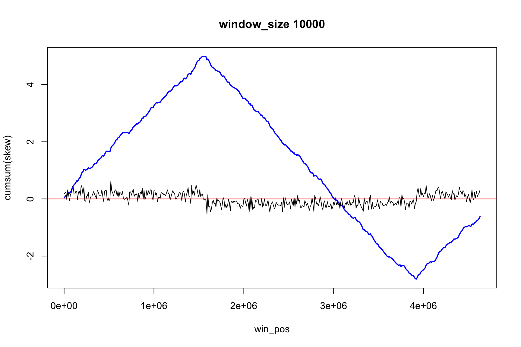
There is an easier way to find Ori
Instead of looking directly at skew, we can look at cumulative skew
\[\text{acc_skew}[i]=\sum_{j=1}^i \text{skew}[j]\]
Now, instead of the change of sign, we look for the minimum and maximum (Why?)
Now it is easier to see the change of sign

The dictionary says
- cumulative
- § (adjective) increasing in quantity, degree, or force by successive additions.
- § increasing, accumulative, growing, mounting; collective, aggregate, amassed.
- § the cumulative effect of two years of drought
- § the effects of pollution are cumulative
Cumulative sum
Everyday you spend some money
Some days you receive money
How much money you have each day?
Cumulative Sum: daily balance
The income can be positive (salary) or negative (expenses)
The balance on first day is your initial money
The balance of today is the balance of yesterday plus the income of today
balance[today] <- balance[yesterday] + income[today]
balance and income are vectors
Since they have different values every day, we represent the income on day i by income[i]
We also represent the balance on day i by balance[i]
The vector income has the values for all days
The element income[i] has the value for a single day
Today and yesterday
We will see several “days”, represented by i
It is useful to think that
irepresents “today”i-1represents “yesterday”
If we know income, we can calculate balance
The balance on first day is your initial money
balance[1] <- income[1]
The balance of today is the balance of yesterday plus the income of today
for(i in 2:length(income)) {
    balance[i] <- balance[i-1] + income[i]
}
Balance looks like this
The same idea applies to GC-skew
The GC skew in each window is like the income in each day
And we want to see the “balance”: cumulative skew
acc_skew[1] <- skew[1]
for(i in 2:length(skew)) {
    acc_skew[i] <- acc_skew[i-1] + skew[i]
}
Same pattern, same solution
How can we calculate acc_skew?
Cumulative skew
It is easy to see that
acc_skew[i]=acc_skew[i-1] + skew[i]
So we can write something like this:
acc_skew[1] <- skew[1]
for(i in 2:length(skew)) {
    acc_skew[i] <- acc_skew[i-1] + skew[i]
}
Can you write this as a function?
Now max & min show the change of sign

Position of the maximum
The maximum value of acc_skew is
max(acc_skew)
[1] 4.9877
It is not really important
We are looking for position, not value of maximum
Position of the maximum
This is the index of the maximum in the acc_skew vector
which.max(acc_skew)
[1] 155
This is always an integer number, between 1 and length(acc_skew)
It is not the position in the genome
Position of the maximum
Since acc_skew vector has the same size as win_pos, we can find the Ori position with this
win_pos[which.max(acc_skew)]
[1] 1540001
win_pos contains the genome positions of each window
This code gives us the position of the window with maximum GC-skew
Locating origin depends on window size
Ori is located in the interval between
win_pos[which.max(acc_skew)]win_pos[which.max(acc_skew)] + size
Skew and Cumulative skew
Skew and Cumulative skew
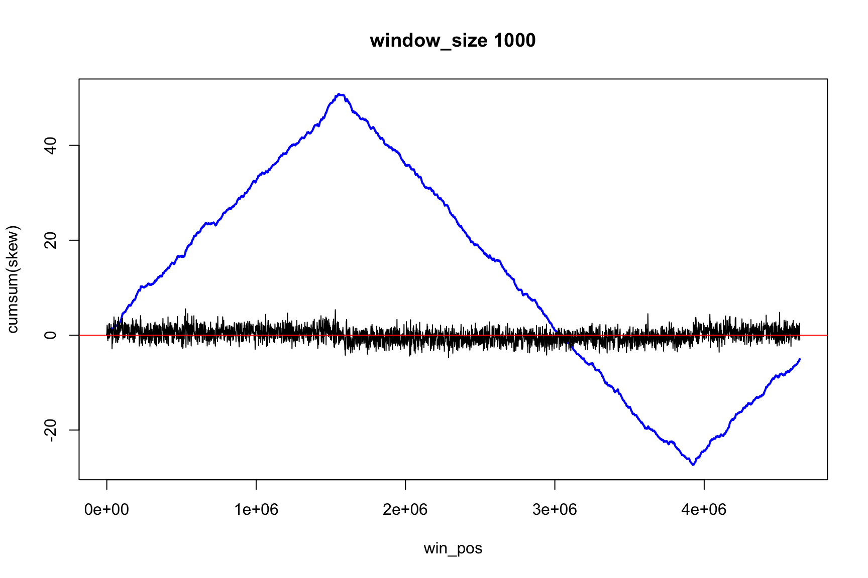
Skew and Cumulative skew
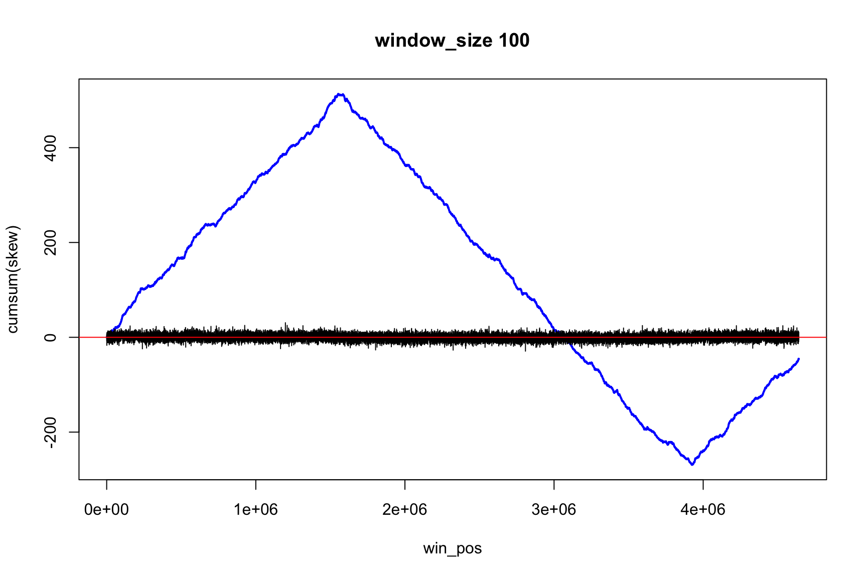
Skew and Cumulative skew

skew changes fast, acc_skew changes slow

Let’s do the same with AT-skew

Last two plots depend on position
First plot is GC-skew versus Position
Second plot is AT-skew versus Position
What is the relationship between GC-skew and AT-skew?
How can you show it?
GC-skew v/s AT-Skew
Have we seen this before?

Cumulative sums are useful
- If we know the income, we can get balance
- If we know the skew, we can get acc_skew
- If we know the change, we can know the state
Systems
Basic Systems Theory
These ideas are useful to understand the reality
A System is a set of parts that interact
Each part can be a smaller system
The behavior of the system depends on the parts AND on the interactions
Total is bigger than the sum of the parts
Complex systems can have emergent properties
That is, the system can do things that the parts cannot
The system is different than each of the parts
A simple system: growing cell lines
In a Petri dish we have one cell
Every hour, 10% of the cells replicate, and they never die
How many cells we have after i hours?
The parts of the system
There is only one element: the cells
There are two values important to them:
- The number of cells
- The change in the number of cells
Let’s give them names
The vector ncells is the number of cells
The value ncells[i] is the number of cells on time i
The vector growth is the growth of the number of cells
There are growth[i] new cells between time i-1 and i
Solving the system
Let’s simulate for 100 hours
First we create empty vectors to store the result
ncells <- rep(NA, 100)
growth <- rep(NA, 100)
Then we start with 1 cell/cm2 and zero growth
ncells[1] <- 1
growth[1] <- 0
Every hour, 10% of the cells replicate
growth[i] <- ncells[i-1]*0.1
The growth on time i depends on the cells existing on time i-1
The number of cells increases
ncells will be the cumulative sum of growth
But growth depends on ncells
Therefore, we calculate both together
Then, time goes by
How many cells we have after 100 hours?
ncells[1] <- 1
growth[1] <- 0
for(i in 2:100) {
    growth[i] <- ncells[i-1]*0.1
    ncells[i] <- ncells[i-1] + growth[i]
}
ncells[100]
[1] 12527.83
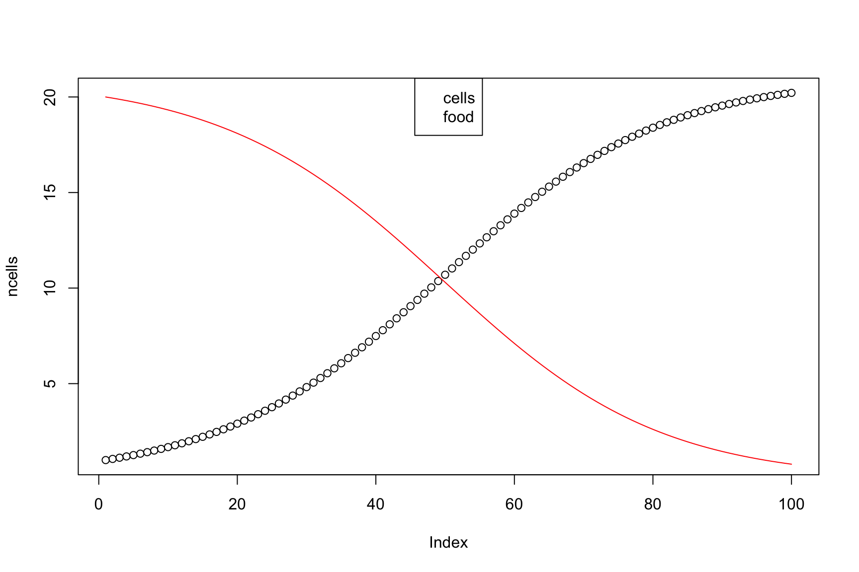
Plot

Limited food
In practice cells never grow that much
There is a limited amount of food
So we need to include food in the system
We represent it with the vector food
Cells eat food, food limits growth rate
Let’s say that initially food[1] <- 20 [ng/uL]
More cells eat more food, limited by the eat_rate:food_change[i] <- ncells[i-1]*food[i-1]*eat_rate
We assume that when a cell gets food, it divides:growth[i] <- ncells[i-1]*food[i-1]*eat_rate
What happens now?
Exercise
Make a program to simulate this system
What happens when food finish?
Is that realistic?
All the code together
ncells <- growth      <- rep(NA, 100)
food   <- food_change <- rep(NA, 100)
ncells[1]      <- 1
growth[1]      <- 0
food[1]        <- 20
food_change[1] <- 0
eat_rate <- 0.003
for(i in 2:100) {
  growth[i]      <-  ncells[i-1]*food[i-1]*eat_rate
  food_change[i] <- -ncells[i-1]*food[i-1]*eat_rate
  ncells[i] <- ncells[i-1] + growth[i]
  food[i]   <-   food[i-1] + food_change[i]
}
Result
Abstraction: avoid fixed numbers
ncells <- growth      <- rep(NA, N)
food   <- food_change <- rep(NA, N)
ncells[1]      <- initial_cells
growth[1]      <- 0
food[1]        <- initial_food
food_change[1] <- 0

for(i in 2:N) {
  growth[i] <- ncells[i-1]*food[i-1]*eat_rate
  food_change[i] <- -ncells[i-1]*food[i-1]*eat_rate
  ncells[i] <- ncells[i-1] + growth[i]
  food[i]   <- food[i-1] + food_change[i]
}