- Decomposition
- breaking down a complex problem or system into smaller parts
- Pattern Recognition
- looking for similarities among and within problems
- Abstraction
- focusing on the important parts only, ignoring irrelevant detail
- Algorithm Design
- developing a step-by-step solution to the problem
March 1st, 2019
Key parts of computational thinking
You can see these when drawing stars
To draw a star, you decompose in these steps:
- hide the turtle
- put the pen down
- point in direction 130 degrees
- repeat 40 times
- move 200 steps
- turn right 130 degrees
Let’s do it
Abstraction: Input
Let’s forget about specific numbers.
In other words, let’s make an abstraction
N: How many sides we will drawangle: how do you turn after each sideR: radius, distance from the center to each peakinitial_angle: initial anglesize: length of each side
Decomposition: Steps
Assuming that you know the input values, you need to:
- Move
Rsteps to the first corner - Point in the direction
initial_angle - repeat
Ntimes- draw a line of length
size - turn right
angledegrees
- draw a line of length
Pattern recognition
In this case it is easy to see a pattern:
- draw a line of length
size - turn right
angledegrees
This pattern is repeated N times
You can do this easily with a loop
Practice
Let’s write a function to draw stars
Hint
initial_anglemust be90+angle/2sizemust be2*R*sin(angle*pi/360)
Question to think: Why these values?
We use R scripts
Last semester we used RMarkdown
This semester we will use R Scripts
Be sure of understanding the difference
We are building R programs, no R documents
Last semester we built documents, like papers and slides
These are files with .Rmd extension
This semester we build programs and scripts
These are files with .R extension
Question What are “file extensions”?
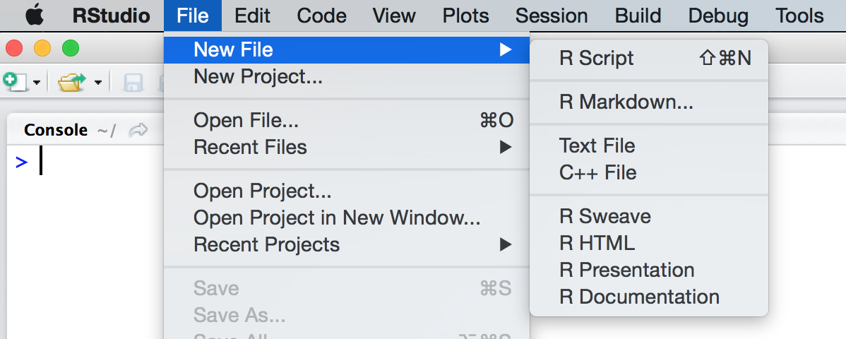
Editing and Executing Code
To create a new file you use the File -> New File menu:
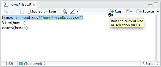
Executing a Single Line
To execute the line of source code where the cursor currently resides you press the Ctrl+Enter key (or use the Run toolbar button):
Executing Multiple Lines
We have seen two ways to execute multiple lines:
Select the lines and press the
Ctrl+Enterkey (or use the Run toolbar button)To run the entire document press the
Ctrl+Shift+Enterkey (or use the Source toolbar button).
Here Source means “run all code from the file”
Source on Save
When editing functions you may wish to set the Source on Save option for the document
Enabling this option will cause the file to automatically be executed every time it is saved
Keyboard Shortcuts
There are many other shortcuts available. Some of the more useful ones are:
Ctrl+Shift+N- New document
Ctrl+O- Open document
Ctrl+S- Save active document
Ctrl+1- Move focus to the Source Editor
Ctrl+2- Move focus to the Console
Bugs
![]()
Bugs
(bəɡ) noun
- a small insect.
- informal a harmful microorganism, as a bacterium or virus.
- an insect of a large order distinguished by having mouthparts that are modified for piercing and sucking.
- a miniature microphone, typically concealed in a room or telephone, used for surveillance.
- an error in a computer program or system.
Debugging with RStudio
Debugging is designed to help you find bugs
To do this, you need to:
- Begin running the code
- Stop the code at the point where you suspect there is a problem
- Walk through the code, step-by-step
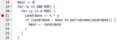
Stopping on a line
Editor breakpoints
The most common way to stop on a line of code is to set a breakpoint.
You can do this by clicking to the left of the line number, or by pressing Shift+F9.
Using the debugger
Once your code stops, you will enter “debug mode”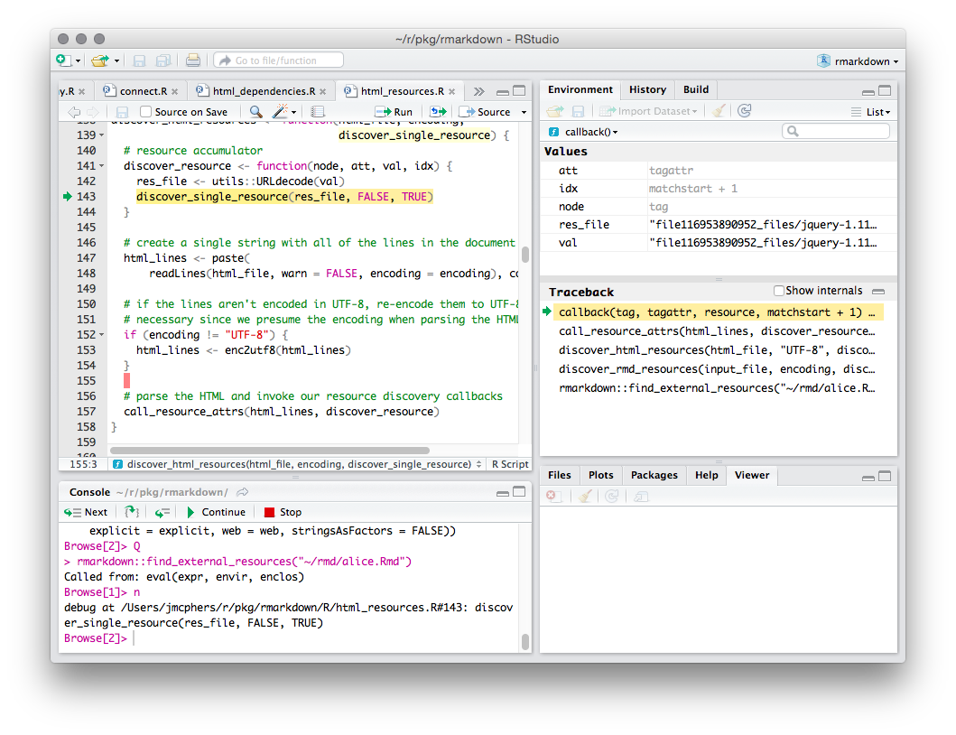
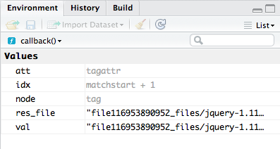
Environment window
Usually in R you’re interacting with the “global environment”
In debug mode, RStudio shows the currently function’s environment
- The objects you see in the Environment pane are in the current function
- Your commands will be evaluated in the context of the function
Environment window
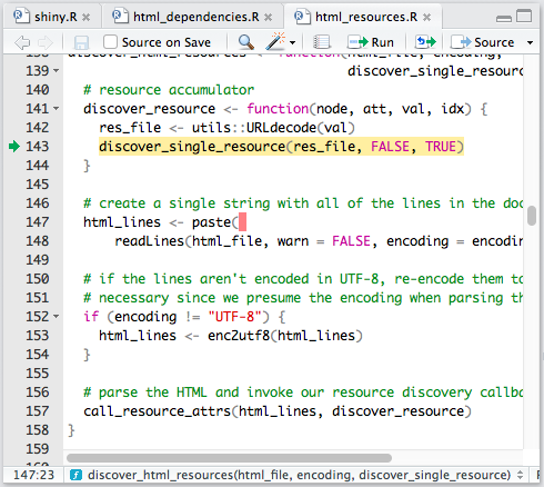
Code window
The code window shows you the currently executing function. The line about to execute is highlighted in yellow
Console
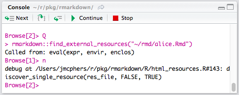
Console
While debugging, you’ll notice two changes to the R console
The first is that the prompt is different:
Browse[1]>
This prompt indicates that you’re inside the R environment browser.
Console
While debugging you can use all the normal commands, plus this:
- Commands are evaluated in the current environment
- If your function has a variable named
x, typingxat the prompt will show you the value of that variable
- If your function has a variable named
- Pressing
Enterat the console will execute the current command and move on to the next one - Several special debugging commands are available
New toolbar on top of the console:

This toolbar provides buttons for debug control commands
- There’s no difference between using the toolbar and entering the commands directly
- learn the command shortcuts
Extra commands when debugging
| Command | Shortcut | Description |
|---|---|---|
n or Enter |
F10 |
Execute next statement |
s |
Shift+F4 |
Step into function |
f |
Shift+F6 |
Finish function/loop |
c |
Shift+F5 |
Continue running |
Q |
Shift+F8 |
Stop debugging |
You can also type help at the Browse[N]> prompt
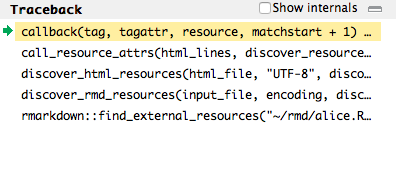
Traceback
The traceback shows you how execution reached the current point,
- from the first function that was run (at the bottom)
- to the function that is running now (at the top).
Stick-person
Draw a head
turtle_right(90)
turtle_forward(4.5)
turtle_left(90)
turtle_forward(9)
turtle_left(90)
turtle_forward(9)
turtle_left(90)
turtle_forward(9)
turtle_left(90)
turtle_forward(4.5)
turtle_right(90)

Arms
# upper body
turtle_forward(9)
turtle_right(180)
turtle_forward(3)
# arms
turtle_left(90)
turtle_forward(9)
turtle_right(90)
turtle_right(90)
turtle_forward(18)
turtle_left(180)
turtle_forward(9)
turtle_left(90)

Draw the first leg
turtle_forward(10)
turtle_forward(5)
# first leg
turtle_right(40)
turtle_forward(10)
turtle_forward(3)
turtle_left(90)
turtle_forward(3)
turtle_left(180)
turtle_forward(3)
turtle_right(40)
turtle_right(50)
turtle_forward(13)

Draw the second leg
# get back to initial angle
turtle_right(40)
turtle_right(90)
turtle_left(10)
turtle_right(20)
# second leg
turtle_left(5)
turtle_left(40)
turtle_forward(13)
turtle_left(90)
turtle_forward(3)
turtle_hide()

Can we simplify it?
Replace repeated pattern by loop
turtle_right(90)
turtle_forward(4.5)
turtle_left(90)
turtle_forward(9)
turtle_left(90)
turtle_forward(9)
turtle_left(90)
turtle_forward(9)
turtle_left(90)
turtle_forward(4.5)
turtle_right(90)
turtle_right(90)
turtle_forward(4.5)
for(i in 1:3) {
    turtle_left(90)
    turtle_forward(9)
}
turtle_left(90)
turtle_forward(4.5)
turtle_right(90)
(use h key)
The size can be variable
turtle_right(90)
turtle_forward(4.5)
for(i in 1:3) {
    turtle_left(90)
    turtle_forward(9)
}
turtle_left(90)
turtle_forward(4.5)
Let’s say size=9 (for now)
turtle_right(90)
turtle_forward(size/2)
for(i in 1:3) {
    turtle_left(90)
    turtle_forward(size)
}
turtle_left(90)
turtle_forward(size/2)
(use h key)
Simplify and generalize the arms
# upper body
turtle_forward(9)
turtle_right(180)
turtle_forward(3)
# arms
turtle_left(90)
turtle_forward(9)
turtle_right(90)
turtle_right(90)
turtle_forward(18)
turtle_left(180)
turtle_forward(9)
turtle_left(90)
# upper body
turtle_forward(size*2/3)


# arms
turtle_right(90)
turtle_forward(size)
turtle_right(180)
turtle_forward(size*2)
turtle_left(180)
turtle_forward(size)
turtle_left(90)
First leg
turtle_forward(10)
turtle_forward(5)
# first leg
turtle_right(40)
turtle_forward(10)
turtle_forward(3)
turtle_left(90)
turtle_forward(3)
turtle_left(180)
turtle_forward(3)
turtle_right(40)
turtle_right(50)
turtle_forward(13)
turtle_forward(15)

# first leg
turtle_right(40)
turtle_forward(13)

turtle_left(90)
turtle_forward(3)
turtle_left(180)
turtle_forward(3)
turtle_right(90)
turtle_forward(13)
Use variable size
turtle_forward(15)
turtle_right(40)
# first leg
turtle_forward(13)
turtle_left(90)
turtle_forward(3)
turtle_left(180)
turtle_forward(3)
turtle_right(90)
turtle_forward(13)
turtle_forward(size*15/9)
turtle_right(40)
# first leg
turtle_forward(size*13/9)
turtle_left(90)
turtle_forward(size/3)
turtle_left(180)
turtle_forward(size/3)
turtle_right(90)
turtle_forward(size*13/9)
Clear code on second leg
# get back to initial angle
turtle_right(40)
turtle_right(90)
turtle_left(10)
turtle_right(20)
# first leg
turtle_left(5)
turtle_left(40)
turtle_forward(13)
turtle_left(90)
turtle_forward(3)
\(40+90-10+20 = 140\)
# get back to initial angle
turtle_right(140)


# first leg
turtle_left(45)

turtle_forward(13)
turtle_left(90)
turtle_forward(3)
Abstraction & decomposition
draw_person <- function(size) {
  draw_head(size*1.2)
  turtle_left(180)
  turtle_forward(size)
  turtle_left(90)
  draw_arm(size*1.5)
  turtle_left(180)
  draw_arm(size*1.5)
  turtle_left(90)
  turtle_forward(size*2)
  turtle_left(20)
  draw_leg(size*2)
  turtle_right(40)
  draw_leg(size*2)
}
This is the main function.
It is my part.
I can change it.
You should not change it.
Instead, you have to provide functions for head, arms and legs.
Body parts
draw_head <- function(size) {
}

draw_arm <- function(size) {
}

draw_leg <- function(size) {
}
This is a Contract
Each part commits to do something
Each part makes a promise
We promise to leave the turtle in the same position as we received it
Let’s start with the arms
You should always start with the easy parts
The easy part may not be the first part
We receive the turtle pointing in the arm direction
We must leave the turtle in the same place and same angle
draw_arm <- function(size) {
    turtle_forward(size)
    turtle_backward(size)
}
From arms to legs
draw_arm <- function(size) {
    turtle_forward(size)


    turtle_backward(size)
}
draw_leg <- function(size) {
    turtle_forward(size)
    turtle_left(90)
    turtle_forward(size/3)
    turtle_backward(size/3)
    turtle_right(90)
    turtle_backward(size)
}
Undoing
Notice that to undo something you have to undo each part in reverse order
You put your socks first, then your shoes
To undo you first “un-put” your shoes, then your socks
In general
\[Undo(A,B,C) = Undo(C), Undo(B), Undo(A)\]
There is another way
Each function has a separate environment with its own variables
We can store position and angle at the start, and reset them at the end
draw_leg <- function(size) {
    old_pos <- turtle_getpos()
    old_angle <- turtle_getangle()
    turtle_forward(size)
    turtle_left(90)
    turtle_forward(size/3)
    turtle_setangle(old_angle)
    turtle_setpos(old_pos[1], old_pos[2])
}
This is useful when the drawing is complex. Keep it in mind
Separation of concerns

We separated the big problem on independent parts
We can change each part without affecting the others, as long as we keep our promises.
For example, you can change the position of the hands, the shape of the head and hands, an others
The code is in stick-person-2.R.
Stick-people in action
Stick-people can explain things well
Stick people are easy to draw
And they are useful
We like seeing people in stories
They make the message more personal
Example: Universal Modeling Language (UML)

Stick people are used in engineering
- to define and communicate
- who are the agents and
- what are the possible actions
on each use case
Example: explaining “Impostor Syndrome”
XKCD Comic

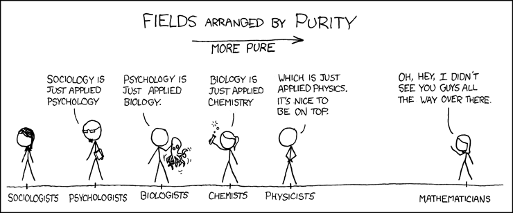
Example: explaining areas of Science
XKCD Comic
There is an xkcd library for R
Creative comics with real data
library(xkcd)
gb <- read.delim("../../2018/cmb2/genbank-size.txt", stringsAsFactors=FALSE)
ratioxy <- diff(range(gb$Release))/diff(range(gb$WGS.Bases))
axes <- xkcdaxis(range(gb$Release), range(gb$WGS.Bases))
axes[[3]]$text$family <- "Humor Sans"

man1 <- xkcdman(aes(x = 140, y = 5.0e+11, scale = 8e+10, ratioxy,
        angleofspine = -1.704265, anglerighthumerus = -0.5807903,
        anglelefthumerus = 3.941945, anglerightradius = 0.0441480,
        angleleftradius = 3.222387, anglerightleg = 5.274786,
        angleleftleg = 4.349295, angleofneck = -1.820286), data=NULL)

man2 <- xkcdman(aes(x = 196, y = 2.8e+11, scale = 8e+10, ratioxy,
        angleofspine = -1.389649, anglerighthumerus = -0.2829418,
        anglelefthumerus = 3.379656, anglerightradius = 0.6164104,
        angleleftradius = 3.073443, anglerightleg = 5.116607,
        angleleftleg = 4.316328, angleofneck = -1.319579), data=NULL)

ggplot(gb, aes(Release,WGS.Bases,label="0")) +
    geom_text(family="Humor Sans", alpha=0.8) + axes + man1 + man2 +
    theme(plot.background = element_blank()) +
    annotate("text", x=160, y=75e10, family="Humor Sans",
        label="Genbank data\nkeeps growing!") +
    xkcdline(aes(x=145, y=5e11, xend=165, yend=65e10),
        data=NULL, xjitteramount = 10)

Faces can illustrate complex data
Invented by Herman Chernoff in 1973
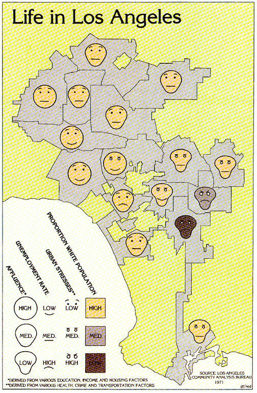
- Humans easily recognize faces and see small changes
- We can show data in the shape of a human face
- Eyes, ears, mouth and nose represent values by their shape, size, placement and orientation
Comics can be used to communicate science
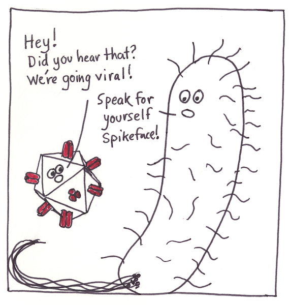
https://doi.org/10.1371/journal.pcbi.1005845.g005
This paper has just been published:
Ten simple rules for drawing scientific comics.
McDermott JE, Partridge M, Bromberg Y
PLoS Computational Biology 14(1) (2018): e1005845.
Homework
Homework 3

I will give you a function called draw_person(size)
Your task is to write the functions draw_head(), draw_arm() and draw_leg().
Then, when you use draw_person(10), you should get a person
This is draw_person(size)
draw_person <- function(size) {
  draw_head(size*1.2)
  turtle_left(180)
  turtle_forward(size)
  turtle_left(90)
  draw_arm(size*1.5)
  turtle_left(180)
  draw_arm(size*1.5)
  turtle_left(90)
  turtle_forward(size*2)
  turtle_left(20)
  draw_leg(size*2)
  turtle_right(40)
  draw_leg(size*2)
}