- DNA sequencing
- Pairwise Alignment
- Genome Assembly
- Multiple Alignment
- Finding Binding Sites
December 17, 2019
Big picture
Genomics
Graphical representation of multiple alignment
A Sequence Logo shows the frequency of each residue and the level of conservation
This is the logo for the multiple alignment of a transcription factor binding site. See www.prodoric.de
Alignment shows what is shared among sequences
We align sequences of some class. The alignment can show what characterizes the class.
From the empirical (position specific) frequencies we can estimate the probability \[\Pr(s_k=\text{"A"}\vert s\text{ is a Binding Site})\] that position \(k\) in sequence \(s\) is an ‘A’, given that \(s\) is a binding site
Conservation is seen on probability
Not all probability distributions are equal. If \[\begin{aligned}\Pr(s_k=\text{"A"}\vert s\in BS)&=\Pr(s_k=\text{"C"}\vert s\in BS)\\ &=\Pr(s_k=\text{"G"}\vert s\in BS)\\&=\Pr(s_k=\text{"T"}\vert s\in BS)\end{aligned}\] then the residue is completely random and we do not know anything. On the other side, if \[\Pr(s_k=\text{"A"}\vert s\in BS)=1 \qquad \Pr(s_k\not=\text{"A"}\vert s\in BS)=0\] then we know everything
Conservation level is measured in bits
Some probability distributions give more information. How much?
We measure information in bits
Since DNA alphabet \(\cal A\) has four symbols we have at most 2 bits per position. The formula is
\[2+\sum_{X\in\cal A}\Pr(s_k=X\vert s\in BS)\log_2 \Pr(s_k=X\vert s\in BS)\]
Using this result to look for more sequences
Basic probability theory says that if \(X\) is any given sequence, then the probability that it is a binding site is \[\Pr(BS\vert X)=\frac{\Pr(X\vert BS)\Pr(BS)}{\Pr(X)}\] Under some hypothesis we also have \[\Pr(X\vert BS)=\Pr(s_1=X_1\vert BS)\Pr(s_2=X_2\vert BS)\cdots\Pr(s_n=X_n\vert BS)\] This is called naive bayes model
Scoring
Using logarithms we will have \[\begin{aligned} \log\Pr(BS\vert X)=\log\frac{\Pr(X\vert BS)}{\Pr(X)}+\log\Pr(BS)\\ \log\Pr(BS\vert X)=\sum_{k=1}^n\log\frac{\Pr(s_k=X_k\vert BS)}{\Pr(s_k=X_k)}+\text{Const.} \end{aligned}\] Thus the sequences that most probably are BS will also have a big value for this formula
Position Specific Scoring Matrices
The score of any sequence \(X\) will be \[\text{Score}(X)=\sum_{k=1}^n\log\frac{\Pr(s_k=X_k\vert BS)}{\Pr(s_k=X_k)}\] So the total score is the sum of the score of each column.
We can write the score function as a \(4\times n\) matrix
These are used to find new binding sites
Exercise
- Go To http://meme-suite.org/
- Use MAST to find all instances of Fur motifs on S.pombe
- What are the differences between FIMO, MAST, MCAST and GLAM2Scan?
- What are the differences between MEME, DREME, MEME-ChIP, GLAM2 and MoMo?
Graphical representation of a motif
A Sequence Logo shows the frequency of each residue and the level of conservation
What is the meaning of the letter’s size?
For any column we have two scenarios. Either
- The nucleotide is random, with probability 0.25
- The nucleotide follows the motif probability
Each scenario has an information content, which we measure in bits \[H=-\sum_{n\in\mathcal A} \Pr(n)\log_2 \Pr(n)\] where \(\mathcal A=\{A,C,T,G\}\). For example \(H_\text{random}=2\)
What is the meaning of the letter’s size?
The size of the letter corresponds to the information gain \[I = H_\text{random} - H_\text{motif}\] For example, if I know the (exact) result of tossing a coin and you don’t, then I know one bit.
If I do not know the exact result but I know that head has probability 88.99721%, then I know 0.5 bits.
The information gain in each column is \[H_\text{random} - H_\text{motif} = 2 + \sum_{n\in\mathcal A} \Pr(n)\log_2 \Pr(n)\]
Finding Binding Sites
If we know the empirical frequencies \(f_{i}(n)\) of the nucleotide \(n\) on each column \(i,\) we can build a position specific score matrix
The score of nucleotide \(n\) at position \(i\) is proportional to \[\log(f_{i}(n)) - \log(F(n))\] where \(F(n)\) is the background frequency of nucleotide \(n\).
But finding the empirical frequencies requires a multiple alignment
How to find motifs without alignment
It is easy to find motifs in a multiple alignment
But we have seen that multiple alignment can be expensive
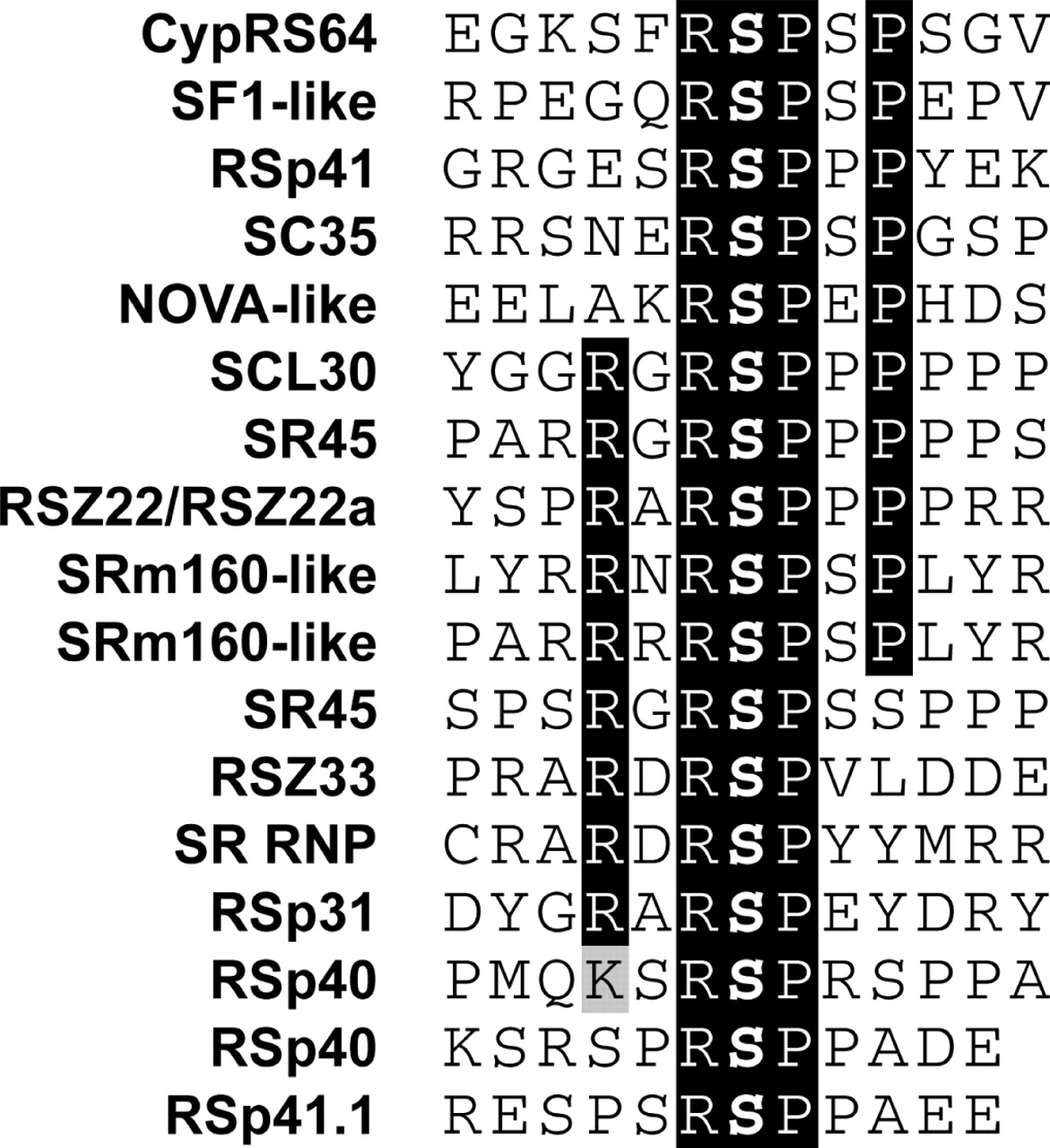
When we are looking for short patterns (a.k.a motifs) we can use other strategies
Nucleic Acids Research, Volume 34, Issue 11, 1 January 2006, Pages 3267–3278, https://doi.org/10.1093/nar/gkl429
Formalization
Given \(N\) sequences of length \(L\): \(seq_1, seq_2, ..., seq_N\), and a fixed motif width \(k,\) we want
- a subsequence of size \(k\) (a \(k\)-mer) that is over-represented among the \(N\) sequences
- or a set of highly similar \(k\)-mers that are over-represented
Testing all sets of \(k\)-mers is computationally intensive, so several heuristics have been proposed
Gibbs Sampling Algorithm
Given \(N\) sequences of length \(L\) and desired motif width \(k\):
- Step 1: Choose a position in each sequence at random: \[a_1 \in seq_1, a_2 \in seq_2, ..., a_N \in seq_N\]
- Step 2: Choose a sequence at random from the set (let’s say, \(seq_j\)).
- Step 3: Make a weight matrix model of width \(k\) from the sites in all sequences except the one chosen in step 2.
- Step 4: Assign a probability to each position in \(seq_j\) using the weight matrix model constructed in step 3: \[p_1, p_2, p_3, ..., p_{L-k+1}\]
Gibbs Sampling Algorithm (cont)
- Step 5: Sample a starting position in \(seq_j\) based on this probability distribution and set \(a_j\) to this new position.
- Step 6: Choose a sequence at random from the set (say, \(seq_{j'}\)).
- Step 7: Make a weight matrix model of width \(k\) from the sites in all sequences except \(seq_{j'}\), but including \(a_j\) in \(seq_j\)
- Step 8: Repeat until convergence (of positions or motif model)
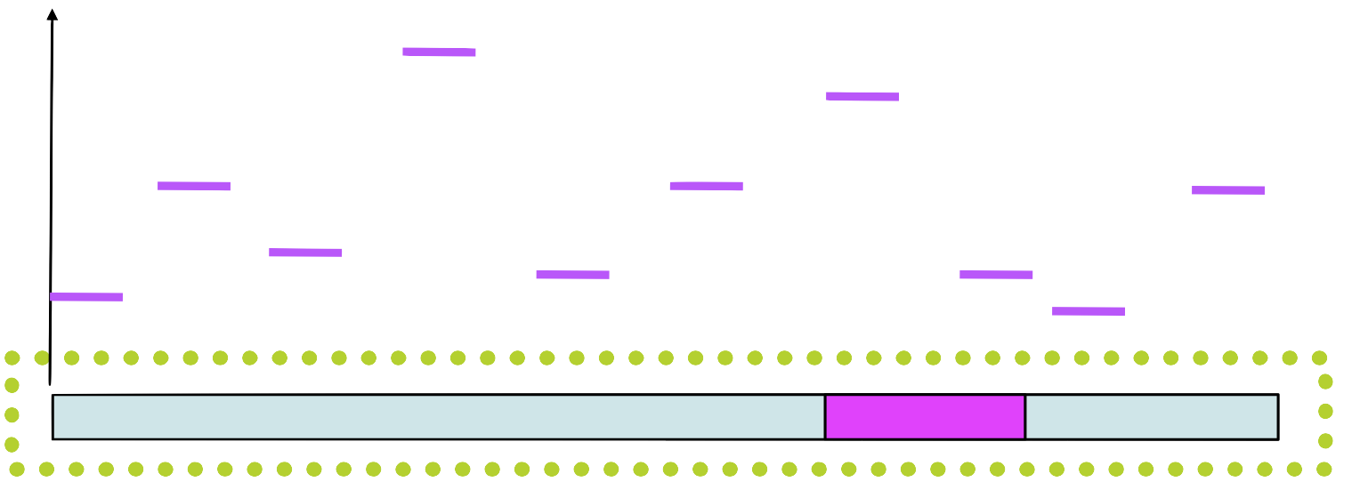
Step 1
Choose a position \(a_i\) in each sequence at random 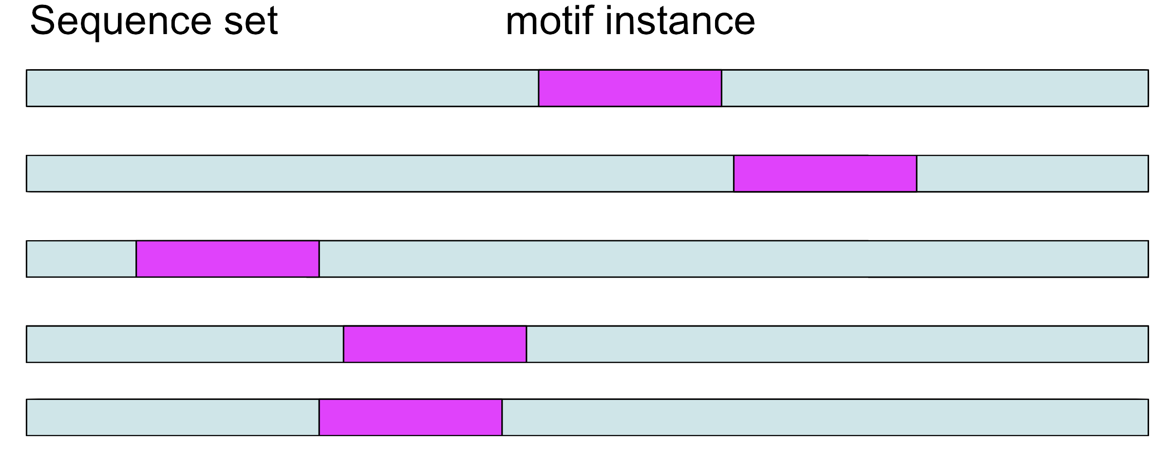
Step 2 and 3
Choose a sequence at random, let’s say \(seq_1.\) Make a weight matrix model from the sites in all sequences except \(seq_1\) 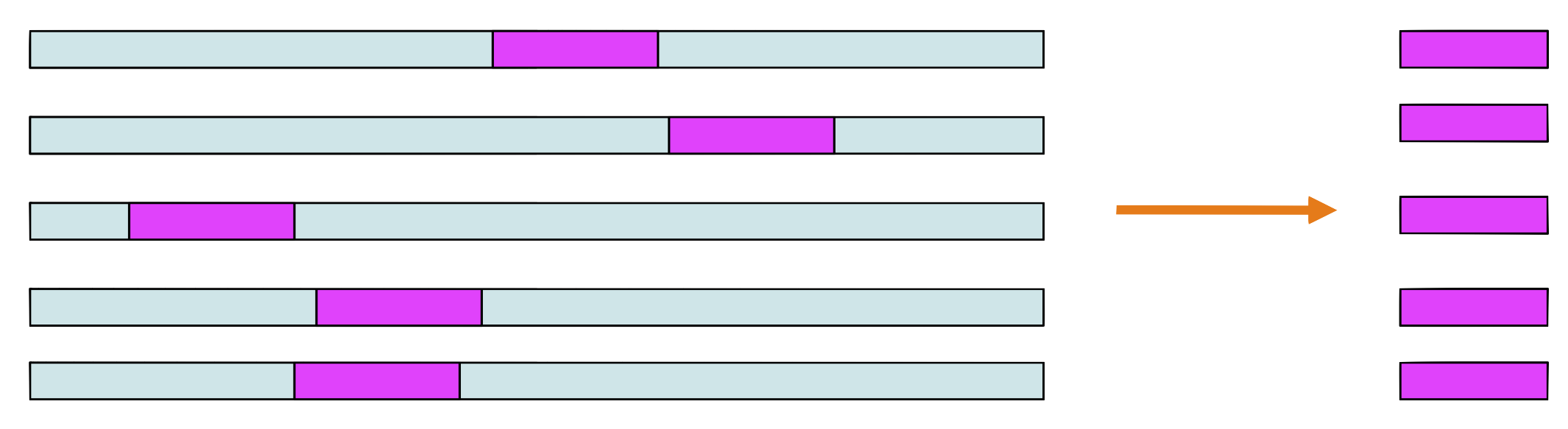
Step 4
Assign a probability to each position in using the weight matrix
Step 5
Choose a new position in \(seq_1\) based on this probability 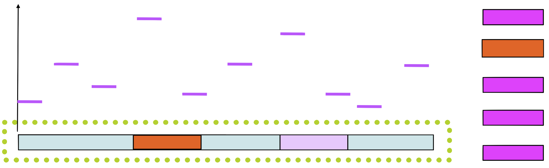
Step 6
Build a new matrix with the new sequence 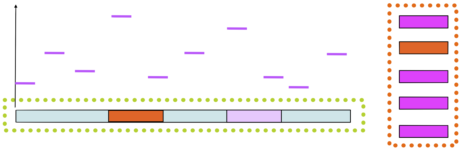
Step 7
Choose randomly a new sequence from the set and repeat 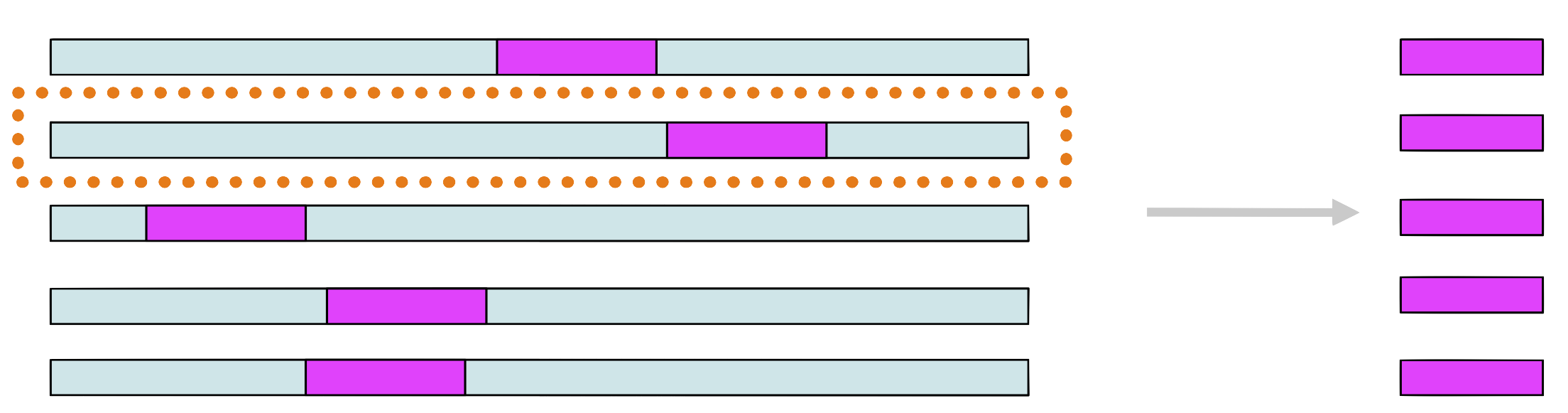
Convergence
We repeat the steps until the matrix no longer changes
Alternative: we stop when the positions \(a_i\) do not change
The methods probably gives us a over-represented motif
Implementation
- Gibbs Motif Sampler Homepage: http://ccmbweb.ccv.brown.edu/gibbs/gibbs.html
- MotifSuite: http://bioinformatics.intec.ugent.be/MotifSuite/Index.htm
- MEME on the MEME/MAST suite
Bioidentification of metagenomic samples
another case for alignment free methods
Context: Metagenomics
Let’s say you get a complex sample:
- Environmental studies
- Human microbiota
- Archeology
You extract total DNA, you sequence all.
You got millions of reads
What is on these reads?
Problem: Identification
Now you ask:
- What are the organisms on this sample?
- How many of them?
- What can they do?
Most of the reads do not align to any reference genome
(most of Prokaryotes have not been isolated)
Two approaches to identify a read
- similarity based: i.e. alignment
- highly specific
- low sensitivity
- composition based: \(k\)-mer frequency
- low specificity
- high sensitivity
Identification without alignment
Given a DNA read \(r\) we want to find which species \(S\) is the most probable origin of the read
We want to find an \(S\) that maximizes \(\Pr(\text{species is }S\vert \text{we saw }r)\)
Thus, the question is how to evaluate this probability. Some approaches:
- Naïve Bayes Classification (Rosen 2008)
- RaiPhy (Nalbantoglu 2011)
Nucleotide composition
Some properties of DNA composition tend to be conserved through evolution
For example, two phylogenetically close species usually have similar GC content
Generalizing the idea, we can consider the relative abundance of
- di-nucleotides
- tri-nucleotides
- and longer oligomers of size \(k\)
An oligomer of size \(k\) is called \(k\)-mer
\(k\)-mers
Given a sequence \(s\) of length \(L\), we characterize it by a vector counting all subwords of size \(k\)
Given a DNA “word” \(w\in {\cal A}^k\) of length \(k\), we define
- Absolute frequency \(n_{(k)}(w;s)=\sum_j[s_j\ldots s_{j+k-1}=w]\)
- Relative frequency \(f_{(k)}(w;s)=n_{(k)}(w;s)/\sum_{v\in\cal A} n_{(k)}(v;s)\)
Remember that \(\mathcal A = \{A,C,G,T\}\) and that \([Q]=1\) iff \(Q\) is true.
How many different k-mers?
The classification must be invariant to reverse complement
The representation should not change if we use either strand
- \(D_k=4^{k/2} + 4[k\text{ even}]\) distinct values
- \(D_k-1\) linearly independent values
- So for \(k=1\) we have only one value: GC content
The question
Given a read \(r\) we want to identify its origin in a set \(\{C_j\}\) of taxas (species, genus, etc.)
We want to compare the probabilities \(\Pr(C_i\vert r)\) for each taxa, and assign \(r\) to the taxa with highest probability
Naïve Bayes Classification
The famous Bayes theorem
Naïve Bayes Classification
The Bayes Part
Using Bayes’ Theorem we can rewrite the unknown in terms of things that we can evaluate
\[\Pr(C_i\vert r)=\frac{\Pr(r\vert C_i)\Pr(C_i)}{\Pr(r)}\]
- \(\Pr(r)\) does not depend on \(S\), so we can ignore it
- \(\Pr(C_i)\) is our a priori idea of \(C_i\) presence
- If we do not know, then we can assume it is constant
Therefore, to maximize \(\Pr(C_i\vert r)\) we need to maximize \(\Pr(r\vert C_i)\)
The Naive Part
The read \(r\) can be seen as a series of overlapping \(k\)-mers (oligomers of size \(k\))
- \(r_1\ldots r_k\)
- \(r_2\ldots r_{k+1}\)
- up to \(r_{L-k}\ldots r_L\)
We naively assume that they are independent, thus \[\Pr(r\vert S)=\Pr(r_1\ldots r_k\vert S)\Pr(r_2\ldots r_{k+1}\vert S)\cdots\Pr(r_{L-k}\ldots r_L\vert S)\]
Now we need to calculate each \(\Pr(r_{i+1}\ldots r_{i+k}\vert S)\)
Prob. of a \(k\)-mer given a specie

Naïve Bayes Classifier
We have therefore \[\Pr(C_j\vert r)=\frac{\Pr(r\vert C_j)\Pr(C_j)}{\Pr(r)} =\prod_i{\Pr(r_i\ldots r_{j+k-1}\vert C_j)}\frac{\Pr(C_j)}{\Pr(r)}\]
where \(\Pr(r)\) is independent of the taxa, and \(\Pr(C_j)\) is usually assumed to be uniform. We can define a score using logarithms
\[\log\Pr(C_j\vert r)=\sum_i{\log\Pr(r_i\ldots r_{j+k-1}\vert C_j)}+\log{\Pr(C_j)}-\log{\Pr(r)}\]
In summary
If we assume that all \(C_i\) are in the same proportion, then \[\text{Score}(C_i|r)=\sum_i \log f_{(k)}(r_i\ldots r_{j+k-1};C_i)\] Therefore, we just need to calculate, for each \(C_i,\) the frequencies \[f_{(k)}(w;C_i)\] for each \(w\in\cal A^k\)
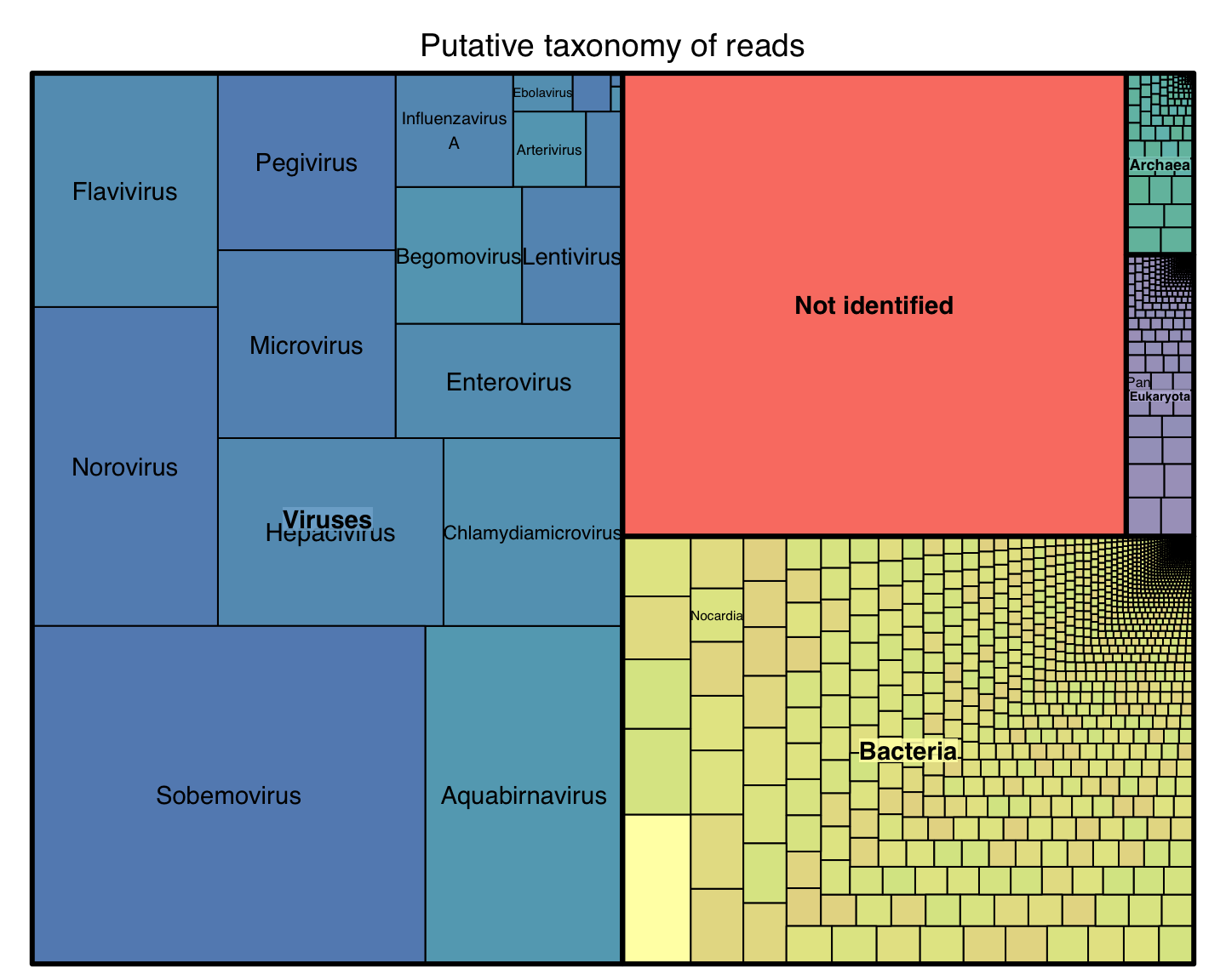
Results with real data
unpublished data from Stockholm University