March 9, 2018
Stick-people in action
Stick-people can explain things well
Despite being easy to draw, stick people are useful
We like seeing people in stories
They make the message more personal
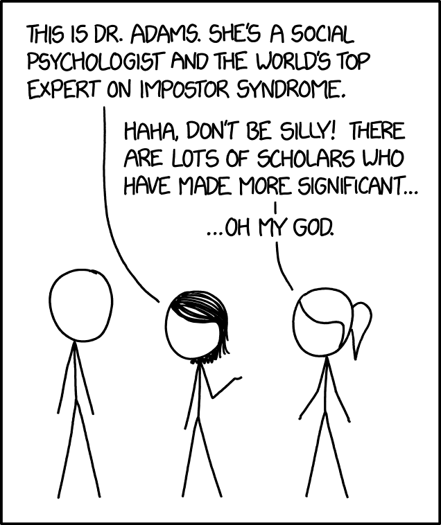
Example: explaining “Impostor Syndrome”
XKCD Comic
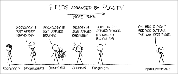
Example: explaining areas of Science
XKCD Comic
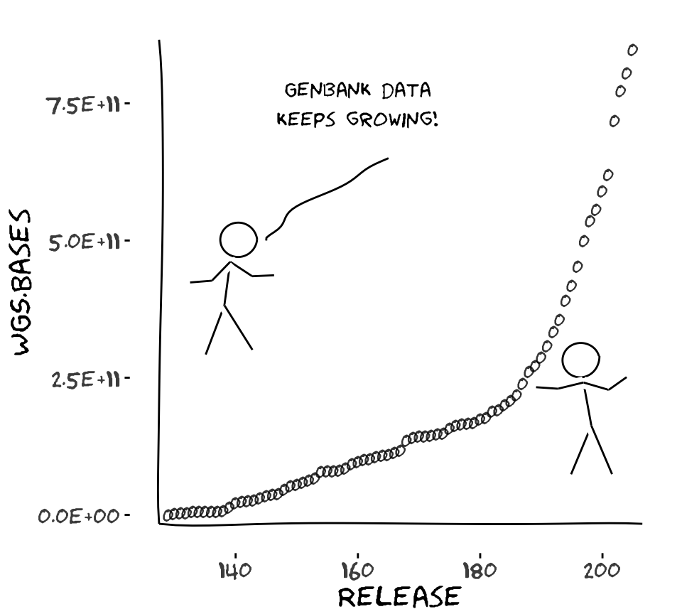
There is an xkcd library for R
Creative comics with real data
library(xkcd)
gb <- read.delim("genbank-size.txt", stringsAsFactors=FALSE)
ratioxy <- diff(range(gb$Release))/diff(range(gb$WGS.Bases))
axes <- xkcdaxis(range(gb$Release), range(gb$WGS.Bases))
axes[[3]]$text$family <- "Humor Sans"

man1 <- xkcdman(aes(x = 140, y = 5.0e+11, scale = 8e+10, ratioxy,
        angleofspine = -1.704265, anglerighthumerus = -0.5807903,
        anglelefthumerus = 3.941945, anglerightradius = 0.0441480,
        angleleftradius = 3.222387, anglerightleg = 5.274786,
        angleleftleg = 4.349295, angleofneck = -1.820286), data=NULL)

man2 <- xkcdman(aes(x = 196, y = 2.8e+11, scale = 8e+10, ratioxy,
        angleofspine = -1.389649, anglerighthumerus = -0.2829418,
        anglelefthumerus = 3.379656, anglerightradius = 0.6164104,
        angleleftradius = 3.073443, anglerightleg = 5.116607,
        angleleftleg = 4.316328, angleofneck = -1.319579), data=NULL)

ggplot(gb, aes(Release,WGS.Bases,label="0")) +
    geom_text(family="Humor Sans", alpha=0.8) + axes + man1 + man2 +
    theme(plot.background = element_blank()) +
    annotate("text", x=160, y=75e10, family="Humor Sans",
        label="Genbank data\nkeeps growing!") +
    xkcdline(aes(xbegin=145, ybegin=5e11, xend=165, yend=65e10),
        data=NULL, xjitteramount = 10)
Faces can illustrate complex data
Invented by Herman Chernoff in 1973
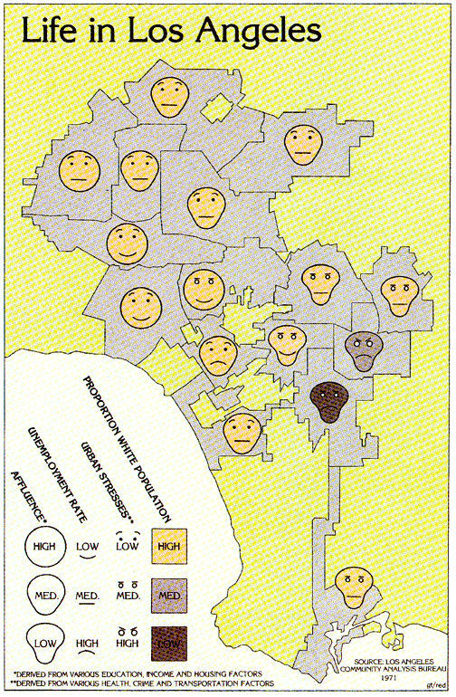
- Show data in the shape of a human face
- Eyes, ears, mouth and nose represent values by their shape, size, placement and orientation
- Humans easily recognize faces and easily notice small changes
- The mapping of features should be careful
- eye size and eyebrow can have significant weight
Comics can be used to communicate science
https://doi.org/10.1371/journal.pcbi.1005845.g005
This paper has just been published:
Ten simple rules for drawing scientific comics.
McDermott JE, Partridge M, Bromberg Y
PLoS Computational Biology 14(1) (2018): e1005845.
Analyzing Biological Sequences in R
For simple cases you can use data from my blog
In most cases we get our sequences from NCBI
NCBI stores all public biological sequences at
https://www.ncbi.nlm.nih.gov/nuccore
Anybody can upload sequences, and they may be wrong
NCBI has a curation process to validate the sequences
If a sequence is good enough to be a reference, then it is stored in the RefSeq collection https://www.ncbi.nlm.nih.gov/refseq
It is easy if you know the Accession Number
Accession numbers are the best way to identify a biological sequence
- Candidatus Carsonella ruddii PV DNA has accession AP009180
- Escherichia coli str. K-12 substr. MG1655 has accession NC_000913
Different sequences can have the same name, but never the same accession
If you do not know the accession use Taxonomy
NCBI search box looks for patterns everywhere, not only on the title
and many sequences can have the same name
To be sure of using the correct sequence, go to NCBI Taxonomy
https://www.ncbi.nlm.nih.gov/taxonomy
Try with “Escherichia coli”. There are many
Once you find the correct species…
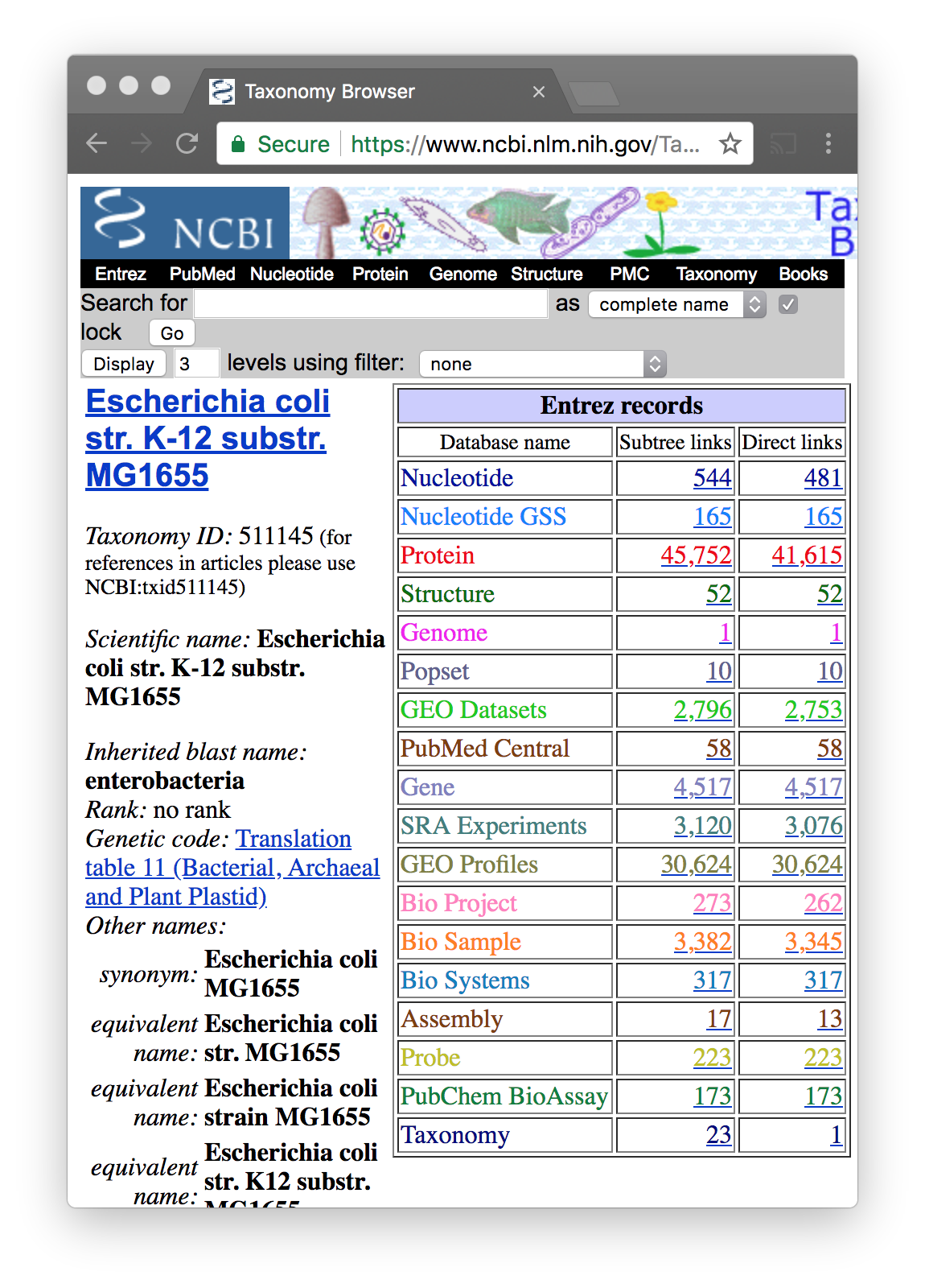
You will see that each organism has a taxonomic ID
You click on Nucleotide–Direct Links
In the search box add the phrase “complete genome”
When you find the correct one..
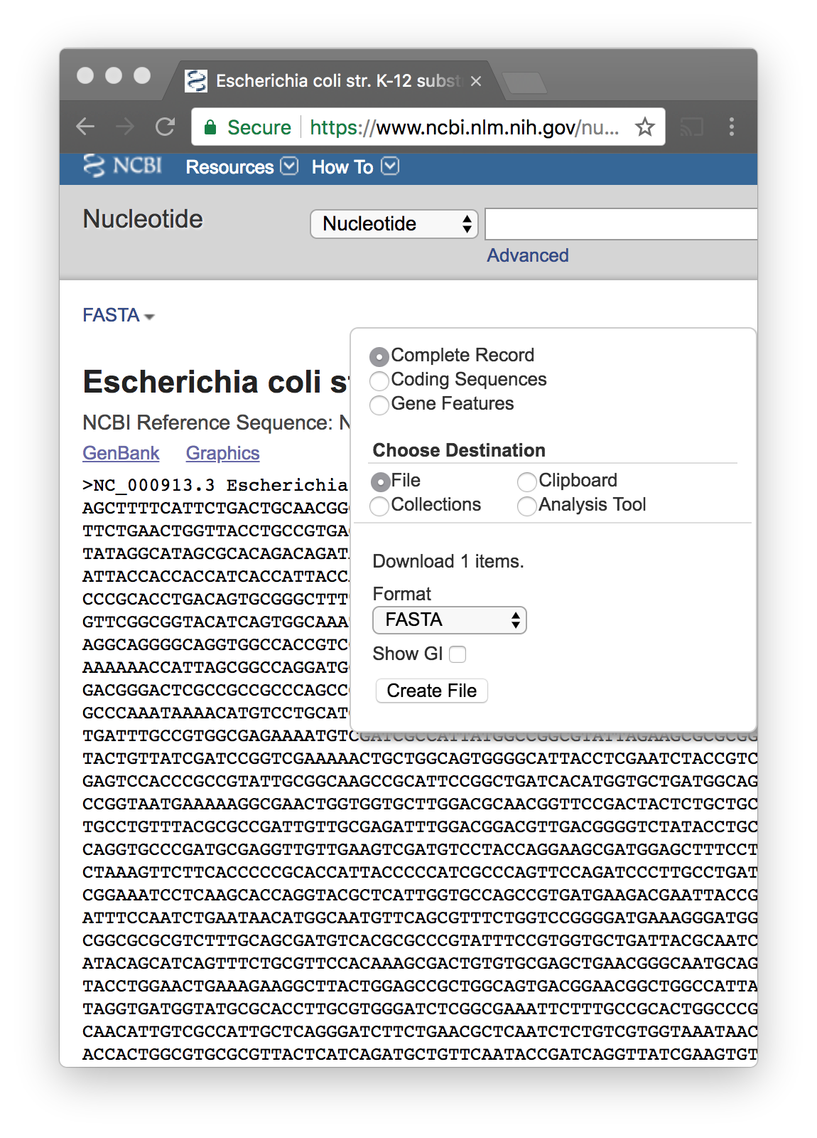
You download the FASTA file
Store it on your computer, and change the name
If you use the Lab’s computers, save it on X:
Reading FASTA in R
To handle sequence data in R, we use the seqinr library
You have to install it once.
install.packages("seqinr")
Then you have to load it on every session
library(seqinr)
read.fasta
read FASTA formatted files
read.fasta(file, seqtype = "DNA", ...)
Inputs
- file
- The name of the file which the sequences in FASTA format are to be read from
- seqtype
- the nature of the sequence: DNA or AA, defaulting to DNA
Output
A list of vectors of chars. Each element is a sequence object.
Example
library(seqinr)
sequences <- read.fasta("NC_000913.fna")
dna <- sequences[[1]]
What have we learned?
What have we learned?
- Some organisms have been sequenced
- We can read the sequences from FASTA files
read.fastareturns a list of vectors of characters- We can create functions to do things with the sequence
- Functions are black boxes with inputs and outputs
- For example we do statistics of the sequence
Why we do statistics on the sequence?
Statistics is a way to tell a story that makes sense of the data
In genomics, we look for biological sense
That story can be global: about the complete genome
Or can be local: about some region of the genome
We will start with global properties
GC-content
From Wikipedia, the free encyclopedia
The percentage of nitrogenous bases on a DNA molecule that are either guanine or cytosine.
- GC content is found to be variable with different organisms.
- The committee on bacterial systematics has recommended use of GC ratios in higher level hierarchical classification
GC-content can be measured by several means
Measuring the melting temperature of the DNA double helix using spectrophotometry
- The absorbance of DNA at a wavelength of 260nm increases when DNA separates into two single strands at melting temperature
Determination of GC content
If the DNA has been sequenced then the GC-content can be accurately calculated by simple arithmetic.
GC-content percentage is calculated as \[\frac{G+C}{A+T+G+C}\]
Exercise 1
Determine the GC content of E.coli
Is this GC content uniform through all genome?
Chargaff’s rules
Discovered by Austrian chemist Erwin Chargaff in 1952
DNA from any cell of all organisms has a 1:1 ratio of pyrimidine and purine bases
The amount of guanine is equal to cytosine and the amount of adenine is equal to thymine.
Elson D, Chargaff E (1952). On the deoxyribonucleic acid content of sea urchin gametes. Experientia 8 (4): 143–145
Chargaff E, Lipshitz R, Green C (1952). Composition of the deoxypentose nucleic acids of four genera of sea-urchin. J Biol Chem 195 (1): 155–160
First Chargaff’s parity rule
A double-stranded DNA molecule globally has percentage base pair equality:
\(\%A = \%T\) and \(\%G = \%C\)
The rigorous validation of the rule constitutes the basis of Watson-Crick pairs
Second Chargaff’s parity rule
Both \(\%A \approx \%T\) and \(\%G \approx \%C\) are valid for each of the two DNA strands
This describes only a global feature of the base composition in a single DNA strand
Exercise 2
Why the first rule is always valid?
How do you determine if \(\%G \approx \%C\)?
Is this valid through all the genome?
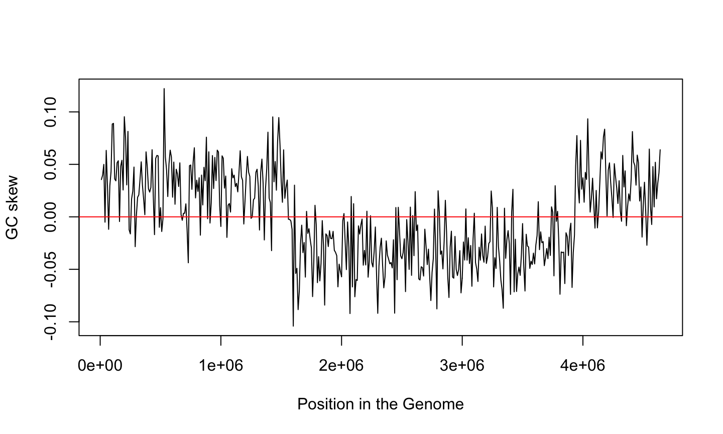
GC Skew
What is the difference \(G-C\) respect to the total \(G+C\)?
Calculate the ratio \[\frac{G-C}{G+C}\] using sliding windows and plot it
What do you see?
Chargaff second rule
In each DNA strand the frequency of occurrence of G is equal to C because the mutation rate is the same
Hence, the second parity rule only exists when there is no mutation or substitution
There is a richness of G over C and T over A in the leading strand
- and vice versa for the lagging strand
GC skew changes sign at the boundaries of the two replichores
This corresponds to DNA replication origin or terminus
What is the story told by GC skew?
Remember Chargaff second rule
For each DNA strand we have \(\%A \approx \%T\) and \(\%G \approx \%C\)
This is because the substitution rate is presumably equal
Hence, the second parity rule only exists when there is no mutation or substitution
But the ratio of G over C is not uniform over the genome
Why?
GC skew and genome replication
GC skew changes sign at the boundaries of the two replichores
This corresponds to DNA replication origin or terminus
The replication origin is usually called ori.
How DNA replicates
How to calculate values on regions
All our calculations are done using functions
What should be
- the output?
- the input(s)?
- the name?
Defining a GC skew function
Remember that an R function is defined like this
name <- function(input1, input2, ...) {
    Calculate
    return(output)
}
The inputs
The GC skew result should depend on:
- the genomic sequence
- the start of the window
- the length of the window
These are the parameters of the function. Do they have
- a name?
- a default value?
The output
How do we transform the input parameters into the output value?
We can use any R function available, such as
seq(from, to, by, length_out)
Task: write a gc_skew function
Applying the function to many values
We want to evaluate gc_skew on different positions of the genome
positions <- seq(from=1, to=length(dna), by= window_size)
How do we apply gc_skew to each element of positions?
Comparative Genometrics
If you want to learn more about the science, read:
Roten C-AH, Gamba P, Barblan J-L, Karamata D. Comparative Genometrics (CG): a database dedicated to biometric comparisons of whole genomes. Nucleic Acids Research. 2002;30(1):142-144