Last Class

December 20, 2018

Other things to do in Rstudio

Other computer languages

You can use other computer languages besides R, such as python

Just write the language at the beginning ```{python}

This calculates the \(e\) number in Python

x=10**50
e=x
for i in range(30):
  x //= (i+1)
  e += x
print(e)

271828182845904523536028747135266237222570213098336

Other languages

You can draw networks from their text description

digraph { size="4,4"; rankdir=LR; bgcolor="transparent";
A->B; A->C; B->C; B->D; D->E; C->E;}

Visualization of matrices

dim(volcano)

[1] 87 61

volcano[1:10,1:10]

      [,1] [,2] [,3] [,4] [,5] [,6] [,7] [,8] [,9]
 [1,]  100  100  101  101  101  101  101  100  100
 [2,]  101  101  102  102  102  102  102  101  101
 [3,]  102  102  103  103  103  103  103  102  102
 [4,]  103  103  104  104  104  104  104  103  103
 [5,]  104  104  105  105  105  105  105  104  104
 [6,]  105  105  105  106  106  106  106  105  105
 [7,]  105  106  106  107  107  107  107  106  106
 [8,]  106  107  107  108  108  108  108  107  107
 [9,]  107  108  108  109  109  109  109  108  108
[10,]  108  109  109  110  110  110  110  109  109
      [,10]
 [1,]   100
 [2,]   101
 [3,]   102
 [4,]   103
 [5,]   103
 [6,]   104
 [7,]   105
 [8,]   106
 [9,]   107
[10,]   108

Image: each values one pixel

Here lower values are red, higher values are white. Like heating metal

image(volcano)

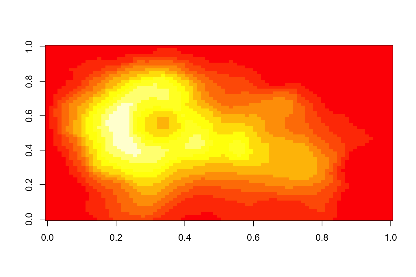
More colors in the same palette

image(volcano, col=heat.colors(100))

Change color palette

image(volcano, col=gray.colors(100))

Image

image(volcano, col=terrain.colors(100))

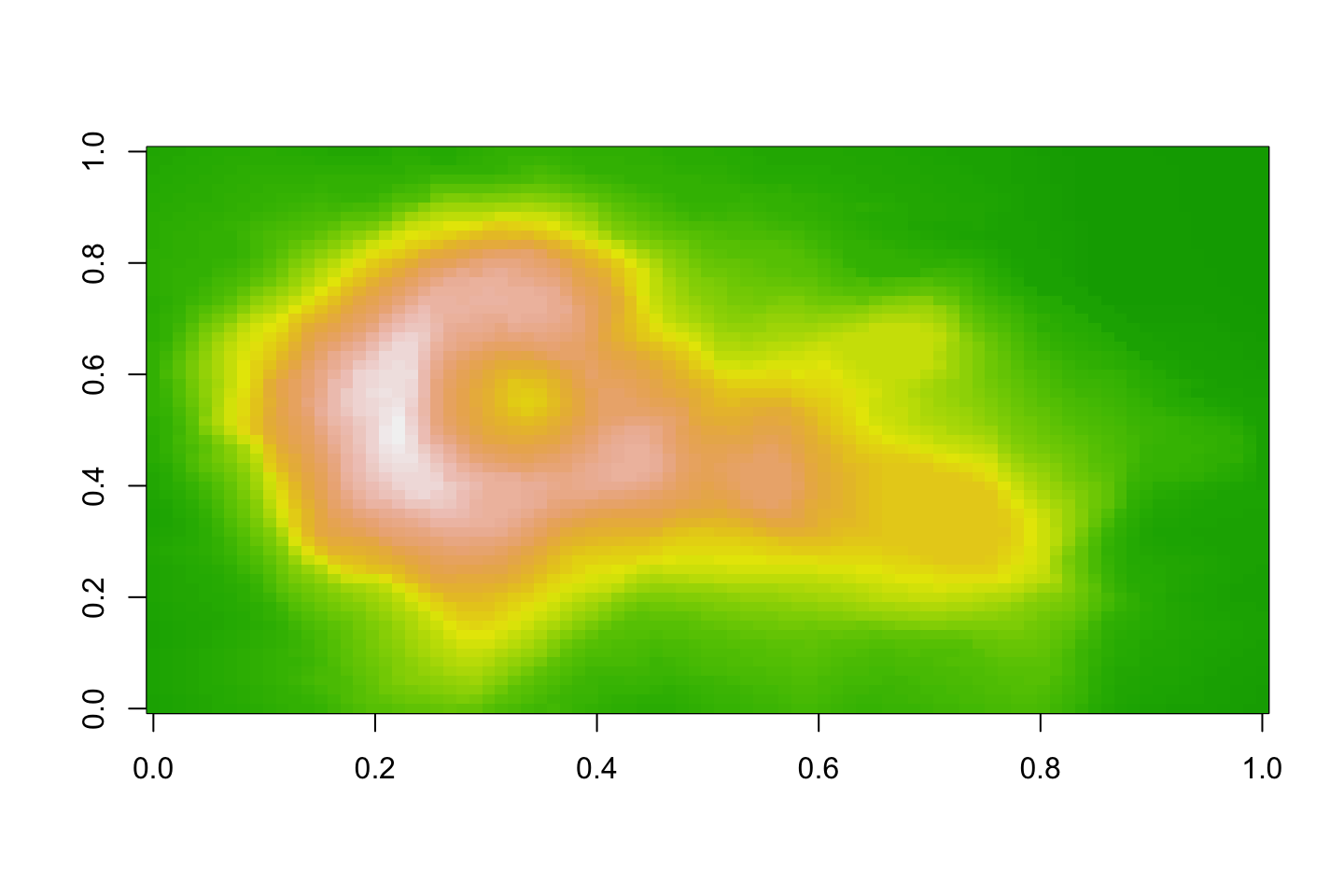
Image

image(volcano, col=topo.colors(100))

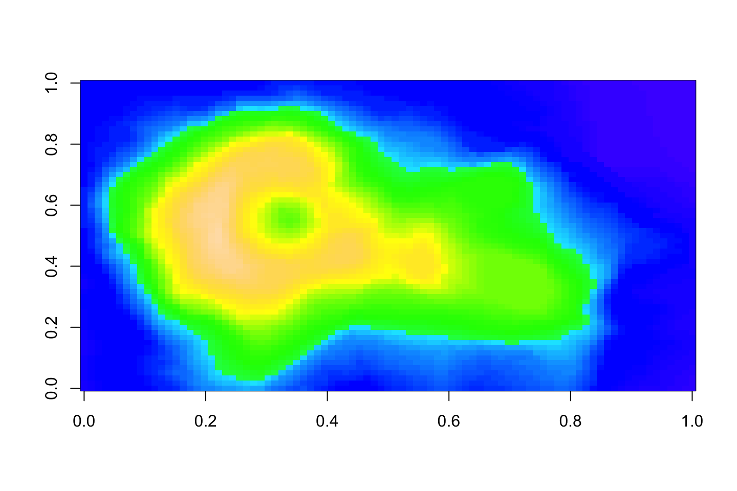
Image

image(volcano, col=cm.colors(100))

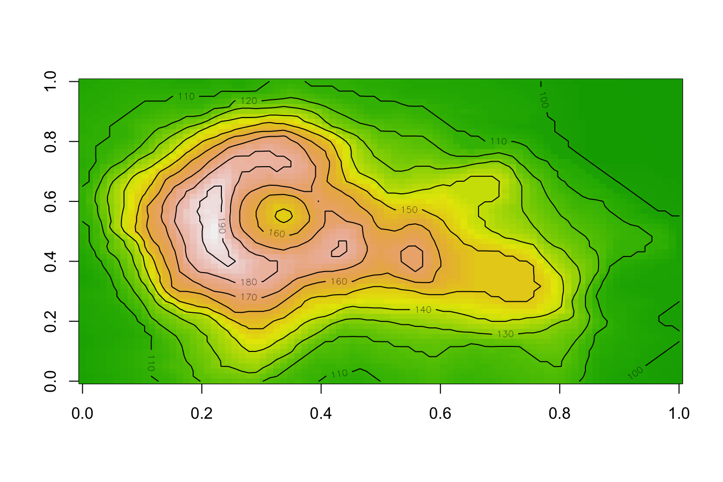
Contour: like a map

contour(volcano)

Image and contour

image(volcano, col=terrain.colors(100))
contour(volcano, add=TRUE)

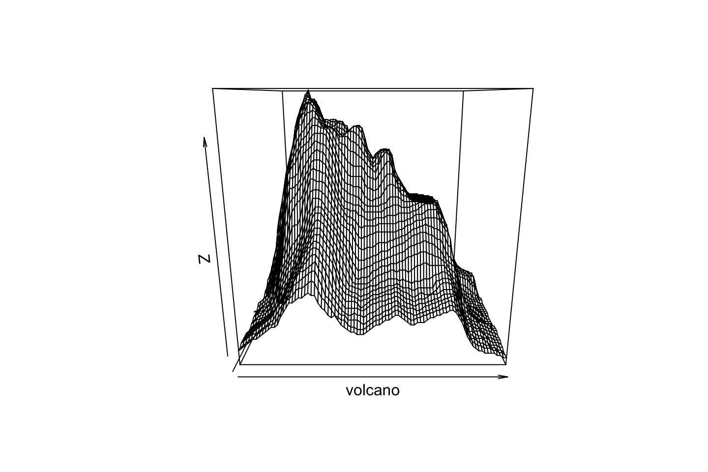
Perspective

persp(volcano)

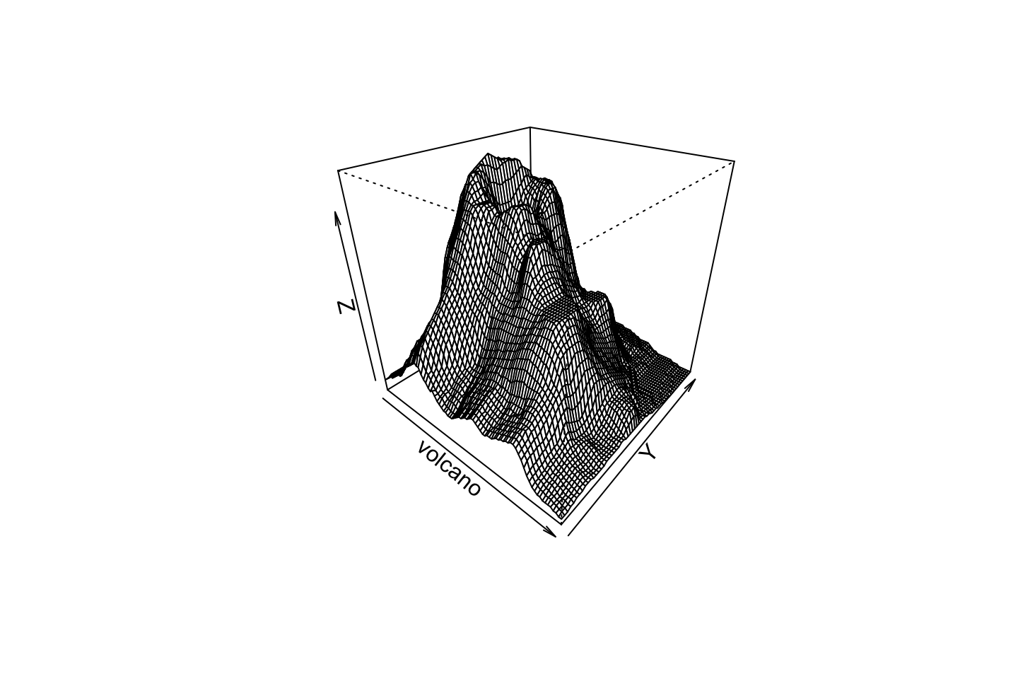
Perspective

persp(volcano, theta=40, phi=30)

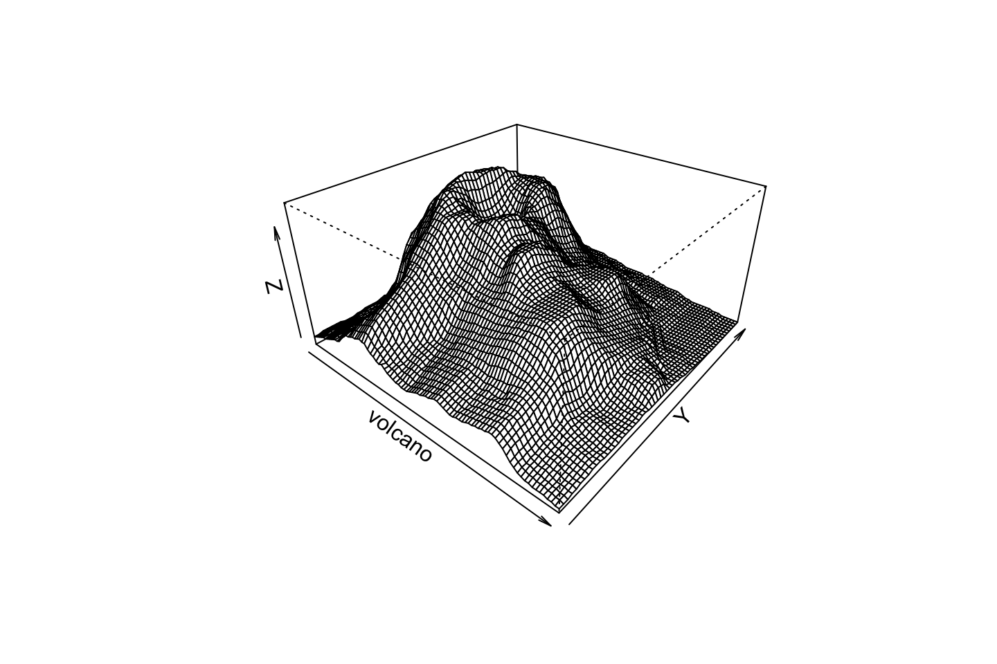
Perspective

persp(volcano, theta=40, phi=30, expand=0.5)

Perspective

persp(volcano, theta=40, phi=30, expand=0.5, col=color[facetcol])

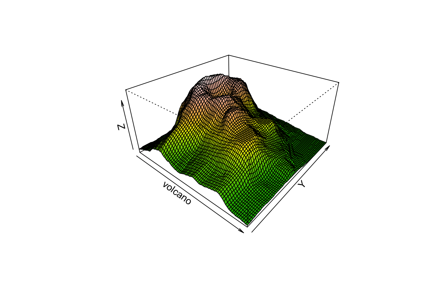
Perspective

persp(volcano, theta=40, phi=30, expand=0.5, col=color[facetcol], border=NA)

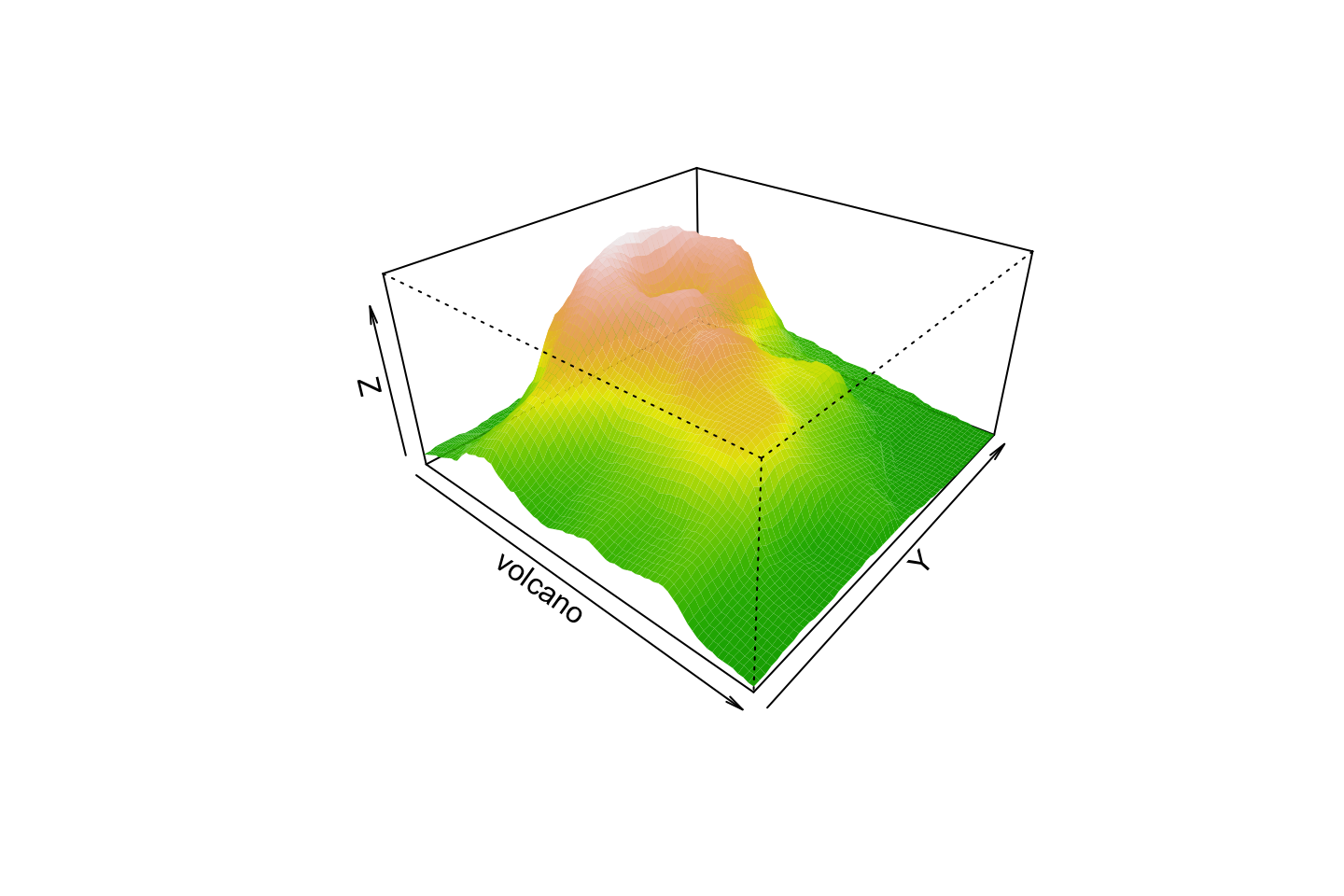
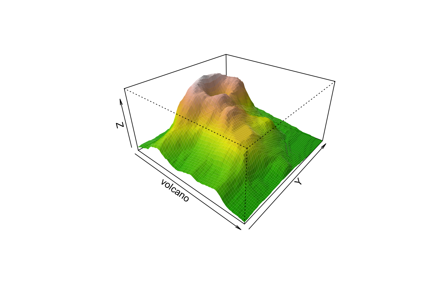
Perspective

persp(volcano, theta=40, phi=30, expand=0.5, col=color[facetcol], border=NA,
      shade=0.5, ltheta=-40, lphi=40)

Make a movie using animation library

You can animate any parameter

Holiday Homework

Learn Sketch (from MIT) and make a game

Quiz solution

Reading data

lib <- read.delim("libraries.txt", header=TRUE)

The data frame can have any name

Can be different from the file name

I choose to have a short name: lib

First step: what are the variables

The caption says

Read mapping percentages of blood and MBD-enriched fecal samples in three libraries

This means PctReadsMappingBaboon, Type and Library

`plot()` is not `barplot()`

plot(PctReadsMappingBaboon ~ ID, data=lib)

These are not bars. We need barplot

`barplot()` is not `plot()`

barplot(PctReadsMappingBaboon ~ ID, data=lib)

Error in barplot.default(PctReadsMappingBaboon ~ ID, data = lib): 'height' must be a vector or a matrix

barplot() does not work wit formulas

It only works with vector, like in the first classes

First plot

barplot(lib$PctReadsMappingBaboon)

Good. We need to separate Libraries, put names, and paint colors

Only library A

barplot(lib$PctReadsMappingBaboon[lib$Library=="A"])

This looks right for the first library

Show also names

barplot(lib$PctReadsMappingBaboon[lib$Library=="A"],
    names.arg = lib$ID[lib$Library=="A"])

Sideway names

barplot(lib$PctReadsMappingBaboon[lib$Library=="A"],
    names.arg = lib$ID[lib$Library=="A"], las=2)

Color depends on Type

barplot(lib$PctReadsMappingBaboon[lib$Library=="A"],
    names.arg = lib$ID[lib$Library=="A"], las=2,
    col=ifelse(lib$Type[lib$Library=="A"]=="blood",
                "red", "brown"))

We better choose the library once

part <- lib[lib$Library=="A",]
barplot(part$PctReadsMappingBaboon,
    names.arg = part$ID, las=2, 
    col=ifelse(part$Type=="blood", "red", "#835923"))

Better separate the library once

barplot(part$PctReadsMappingBaboon, names.arg = part$ID, 
    col=ifelse(part$Type=="blood", "red", "#835923"),
     ylim=c(0,100), las=2)

Red line is mean of Pct for `Type=="blood"`

red_l <- mean(lib$PctReadsMappingBaboon[lib$Type=="blood"])
red_l

[1] 85.52833

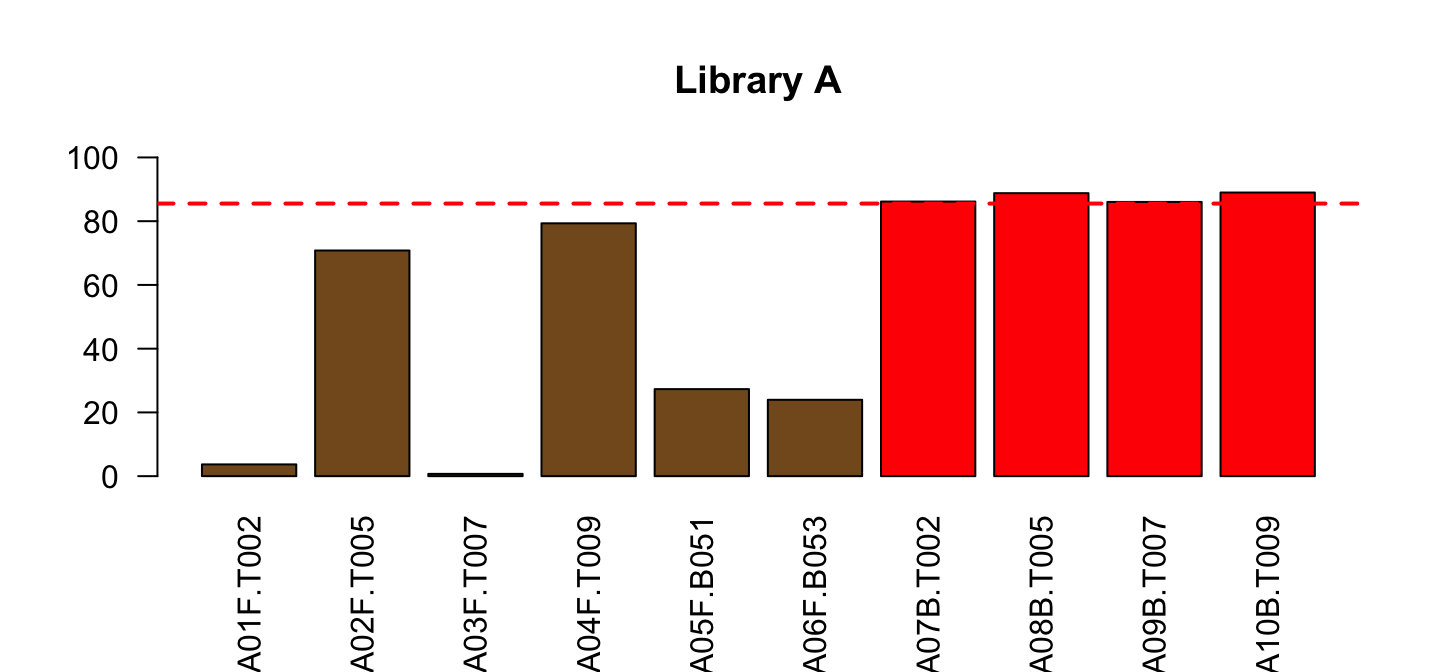
Draw the dashed line

part <- lib[lib$Library=="A",]
barplot(part$PctReadsMappingBaboon, names.arg = part$ID, 
    col=ifelse(part$Type=="blood", "red", "#835923"),
     ylim=c(0,100), las=2, main="Library A")
abline(h=red_l, col="red", lty=2, lwd=2)

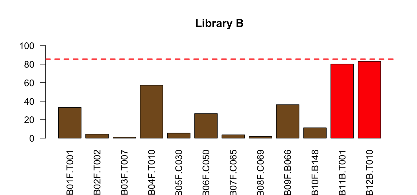
Do the same for Library B

part <- lib[lib$Library=="B",]
barplot(part$PctReadsMappingBaboon, names.arg = part$ID, 
    col=ifelse(part$Type=="blood", "red", "#835923"),
     ylim=c(0,100), las=2, main="Library B")
abline(h=red_l, col="red", lty=2, lwd=2)

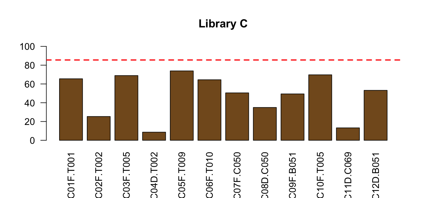
Do the same for Library C

part <- lib[lib$Library=="C",]
barplot(part$PctReadsMappingBaboon, names.arg = part$ID, 
    col=ifelse(part$Type=="blood", "red", "#835923"),
     ylim=c(0,100), las=2, main="Library C")
abline(h=red_l, col="red", lty=2, lwd=2)

All together (see example)

par(mfrow=c(3,1))
part <- lib[lib$Library=="A",]
barplot(part$PctReadsMappingBaboon, names.arg = part$ID,
    las=2, ylim=c(0,100), 
    col=ifelse(part$Type=="blood","red","#835923"))
abline(h=red_l, col="red", lty=2, lwd=2)
part <- lib[lib$Library=="B",]
barplot(part$PctReadsMappingBaboon, names.arg = part$ID,
    las=2, ylim=c(0,100), 
    col=ifelse(part$Type=="blood","red","#835923"))
abline(h=red_l, col="red", lty=2, lwd=2)
part <- lib[lib$Library=="C",]
barplot(part$PctReadsMappingBaboon, names.arg = part$ID,
    las=2, ylim=c(0,100), 
    col=ifelse(part$Type=="blood","red","#835923"))
abline(h=red_l, col="red", lty=2, lwd=2)
par(mfrow=c(1,1))

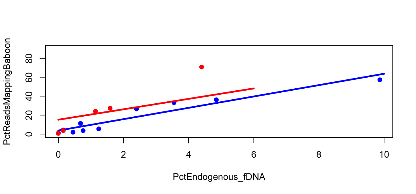
Figure 2

Figure 2 for library B

plot(PctReadsMappingBaboon ~ PctEndogenous_fDNA, data=lib, 
     subset=Type=="feces" & Library=="B", pch=19, col="blue")

Linear model for the line

model_B <- lm(PctReadsMappingBaboon ~ PctEndogenous_fDNA,
    data=lib, subset=Type=="feces" & Library=="B")

use the same formula, data and subset as in plot()

Predict the line for new data

x_B <- 0:10
y_B <- predict(model_B,
    newdata = data.frame(PctEndogenous_fDNA=x_B))

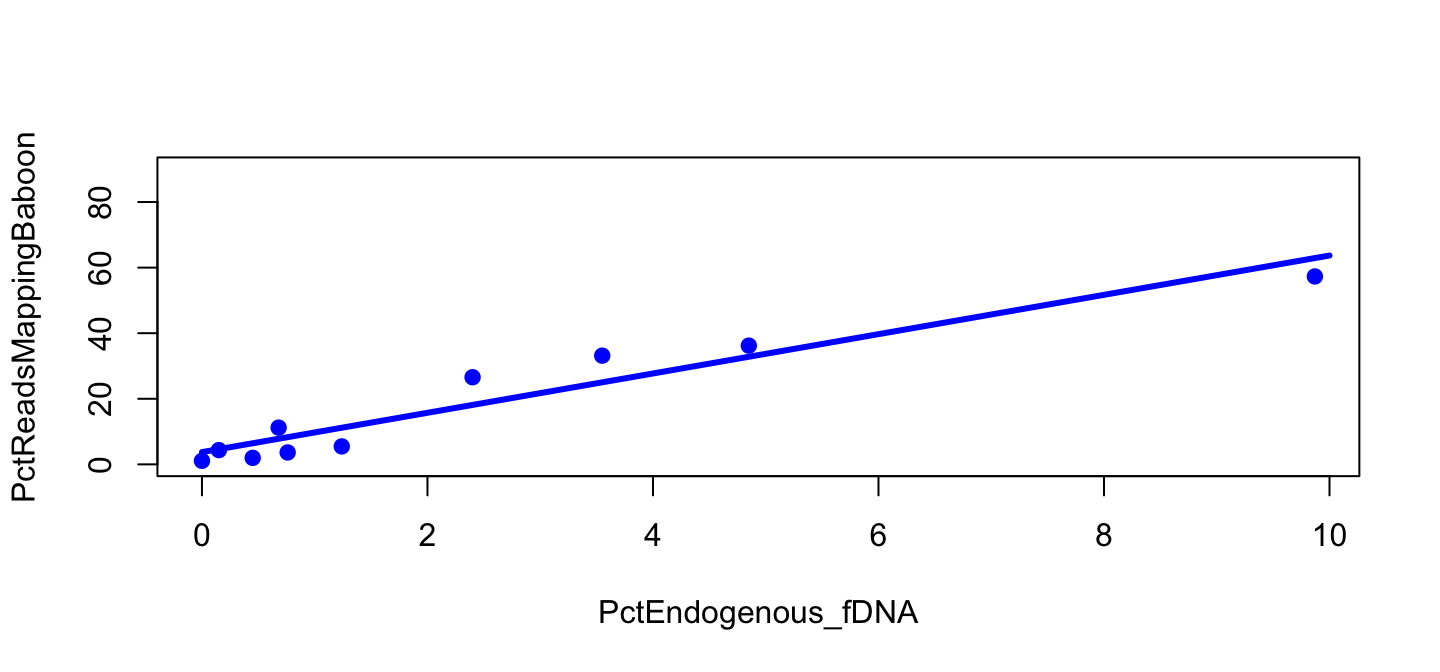
Figure 2 with line

plot(PctReadsMappingBaboon ~ PctEndogenous_fDNA,
     data=lib, subset=Type=="feces" & Library=="B",
     pch=19, col="blue", ylim=c(0,90))
lines(y_B ~ x_B, col="blue", lwd=3)

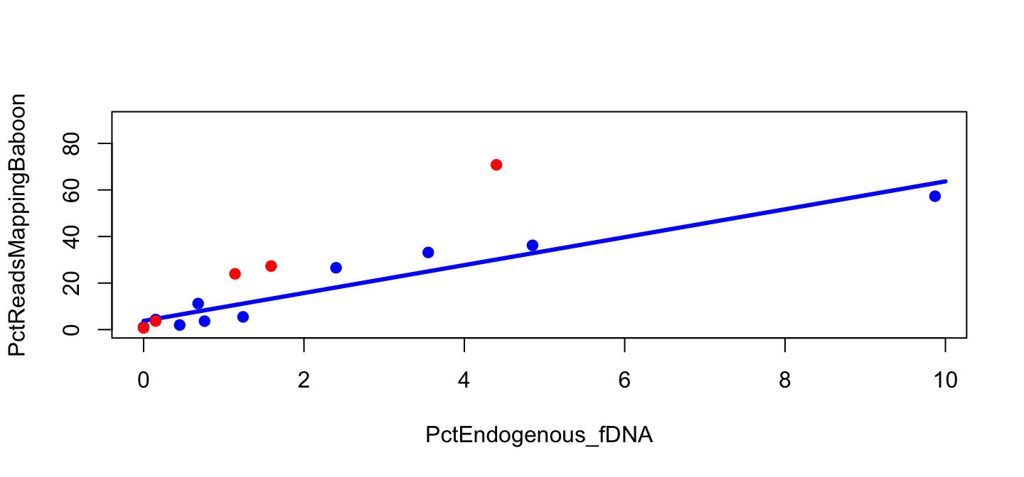
Points for Library A

plot(PctReadsMappingBaboon ~ PctEndogenous_fDNA,
     data=lib, subset=Type=="feces" & Library=="B",
     pch=19, col="blue", ylim=c(0,90))
lines(y_B ~ x_B, col="blue", lwd=3)
points(PctReadsMappingBaboon ~ PctEndogenous_fDNA,
     data=lib, subset=Type=="feces" & Library=="A",
     pch=19, col="red")

Model for Library A

model_A <- lm(PctReadsMappingBaboon ~ PctEndogenous_fDNA,
    data=lib, subset=Type=="feces" & Library=="A")
x_A <- 0:6
y_A <- predict(model_A,
    newdata=data.frame(PctEndogenous_fDNA=x_A))

Finally, plot everything

plot(PctReadsMappingBaboon ~ PctEndogenous_fDNA,
     data=lib, subset=Type=="feces" & Library=="B",
     pch=19, col="blue", ylim=c(0,90))
lines(y_B ~ x_B, col="blue", lwd=3)
points(PctReadsMappingBaboon ~ PctEndogenous_fDNA,
     data=lib, subset=Type=="feces" & Library=="A",
     pch=19, col="red")
lines(y_A ~ x_A, col="red", lwd=3)

Other things to do in Rstudio

Other computer languages

Other languages

Visualization of matrices

Image: each values one pixel

More colors in the same palette

Change color palette

Image

Image

Image

Contour: like a map

Image and contour

Perspective

Perspective

Perspective

Perspective

Perspective

Perspective

Make a movie using animation library

You can animate any parameter

Holiday Homework

Learn Sketch (from MIT) and make a game

Quiz solution

Reading data

First step: what are the variables

plot() is not barplot()

barplot() is not plot()

First plot

Only library A

Show also names

Sideway names

Color depends on Type

We better choose the library once

Better separate the library once

Red line is mean of Pct for Type=="blood"

Draw the dashed line

Do the same for Library B

Do the same for Library C

All together (see example)

Figure 2

Figure 2 for library B

Linear model for the line

Predict the line for new data

Figure 2 with line

Points for Library A

Model for Library A

Finally, plot everything

`plot()` is not `barplot()`

`barplot()` is not `plot()`

Red line is mean of Pct for `Type=="blood"`