December 6, 2018
About Quiz 4
Quiz results
- 43 people attended the quiz
- 23 persons delivered their answers
- 20 lazy ones
- 17 wrote their student number
- 15 wrote their number in the correct format
What is the correct format?
Plots: bad ideas
plot(sra):- plots all the data frame
plot(day~log(bases), data = sra):- sideways
plot(log(bases)~log(day), data=sra):- log-log, not semi-log
Good plots
plot(bases~day, data=sra, log="y")- Publication Quality
plot(log(bases) ~ day, data = sra)- Good for analysis
Modelling genomic databases
13 persons did the model. All of them did it well
Two people did exp(coef(model)[2])
But nobody explained the meaning
Meaning (of life)
sra <- read.table("sra_bases.txt", header=TRUE)
model <- lm(log(bases) ~ day, data=sra)
model
Call:
lm(formula = log(bases) ~ day, data = sra)

Coefficients:
(Intercept)          day
   28.34146      0.00248
Coefficients are log(bases)
In a semi-log model, we have \[\log(\text{bases}) = \underbrace{\log(\text{initial})}_{\texttt{coef(model)[1]}} + \underbrace{\log(\text{rate})}_{\texttt{coef(model)[2]}} \cdot \text{days}\]
Undoing log(), we have \[\text{bases} = \text{initial}\cdot\text{rate}^\text{days}\]
Thus, \(\text{rate}=\)exp(coef(model)[2])\(=1.0025\)
Meaning of rate
If \(\text{rate}=1.0025\) it means that the database grows \(0.2486\%\) every day
- That is \(147.5\%\) every year
- That is \(295\%\) in two years
Predicting the future
To make predictions using the model, we usepredict(model, newdata)
We need a data frame with one column named day, because we used day in the formula
The last day in sra is max(sra$day)
Two years after the last will be max(sra$day) + 2 * 365
so newdata=data.frame(day = max(sra$day) + 2 * 365)
Why we do quizzes
- To rehearse the exam procedures
- To test your learning
- To do realistic work
- To see if you can follow simple instructions
- To find which of you will be good scientist
Quizzes are important if you want to succeed
How to analyze the “free fall” experiment
An ideal falling ball
| height | speed | time |
|---|---|---|
| 2.0000 | -0.20 | 0.0001 |
| 1.9778 | -0.69 | 0.0496 |
| 1.9310 | -1.18 | 0.0988 |
| 1.8598 | -1.67 | 0.1505 |
| 1.7640 | -2.16 | 0.2002 |
| 1.6438 | -2.65 | 0.2509 |
| 1.4990 | -3.14 | 0.2976 |
| 1.3297 | -3.63 | 0.3505 |
| 1.1360 | -4.12 | 0.3991 |
| 0.9177 | -4.61 | 0.4512 |
| 0.6750 | -5.10 | 0.5004 |

What is the good formula this time?
We can use a logarithmic scale to see if we get a straight line
- If we get straight line in semi-log then the formula is \[y=A\cdot B^x\]
- If we get straight line in log-log then the formula is \[y=A\cdot x^B\]
Logarithmic scale


This is not any exponential
There are many possible functions that connect \(x\) and \(y\)
We will try a polynomial formula
A polynomial is a formula like \[y=A + B\cdot x + C\cdot x^2 +\cdots+ D\cdot x^n\]
The highest exponent is the degree of the polynomial
We will try a 2-degree formula \[\text{height}=A+B\cdot\text{time}+C\cdot\text{time}^2\]
A new column for polynomial model
We need to add an extra column, with the square of the time
ball$time_sq <- ball$time^2
head(ball)
  height speed    time   time_sq
1  2.000 -0.20 0.00010 1.000e-08
2  1.978 -0.69 0.04962 2.462e-03
3  1.931 -1.18 0.09878 9.757e-03
4  1.860 -1.67 0.15047 2.264e-02
5  1.764 -2.16 0.20016 4.007e-02
6  1.644 -2.65 0.25093 6.296e-02
We really have to add a new column
You may be tempted to use
model <- lm(height ~ time^2, data=ball)
But that does not work.
Exponents and multiplications in formulas have a different meaning
(that we will see later)
Linear model for polynomial
Now we use two independent variables in the model. This is different from the plot() function
model <- lm(height ~ time + time_sq, data=ball)
model
Call:
lm(formula = height ~ time + time_sq, data = ball)

Coefficients:
(Intercept)         time      time_sq
      1.999       -0.187       -4.929
Interpretation
We used the formula \[\text{height}=A+B\cdot\text{time}+C\cdot\text{time}^2\] The linear model gave us \[\begin{aligned} A&=2\\ B&=-0.187\\ C&=-4.9 \end{aligned}\]
Predicted v/s original
plot(height ~ time, data=ball)
lines(predict(model) ~ time, data=ball, col="red")

It works!
Real values are near
Our experimental data has a margin of error
Also, the points are not exactly on the line
Thus, the model’s coefficients have a margin of error
coef(model) shows only the average
To see the confidence intervals, we use confint()
Confidence Intervals
confint(model)
              2.5 %  97.5 %
(Intercept)  1.9927  2.0053
time        -0.2364 -0.1386
time_sq     -5.0077 -4.8504
According to our experiment, the real values are probably within the shown ranges
Confidence Intervals
confint(model)
              2.5 %  97.5 %
(Intercept)  1.9927  2.0053
time        -0.2364 -0.1386
time_sq     -5.0077 -4.8504
NOTE: in this case
- the real
(Intercept)is 2.0, - the real coefficient for
timeis 0.2 - the real coefficient for
time_sqis -4.9
Our experiment
Some results
seconds   position   replica
132          10         1
208          20         1
261          30         1
336          40         1
364          50         1
443          60         1
469          70         1
522          80         1
523          90         1
132          10         2
207          20         2
261          30         2
337          40         2
363          50         2
444          60         2
471          70         2
525          80         2
526          90         2
Wrong result
seconds position        replica
0       0       1
82      19      1
184     38      1
260     57      1
315     76      1
366     95      1
417     114     1
469     133     1
487     152     1
507     171     1
0       0       2
109     19      2
217     38      2
295     57      2
351     76      2
397     95      2
465     114     2
484     133     2
509     152     2
550     171     2
This is not correct
The data must be exactly what we observe
Later we can transform it for the analysis
Raw data is sacred
Keep it true
Replicas
Every serious experiment should be repeated at least 3 times
Without replication, it can be wrong
Replicas indicate that the result is repetible
Technical and biological replicas
In molecular biology we have two kinds of replicas
- Technical replicas
- the same organism, measured several times
- Biological replicas
- different organisms, measured at least one time
Technical and biological replicas
Technical replicas give you precise measurements of a single individual
This is what we do in Medicine
Biological replicas gives you data about one or more species
That is what we do in Science
Energy
We can also model position v/s speed
plot(height ~ speed,
     data=ball)

plot(log(height) ~ speed,
     data=ball)

Another polynomial model
Logarithmic scale does not show a straight line. We add another column to use a polynomial model
ball$speed_sq <- ball$speed^2
model2 <- lm(height ~ speed + speed_sq, data=ball)
coef(model2)
(Intercept)       speed    speed_sq
  2.002e+00   2.566e-14  -5.102e-02
Confidence intervals
confint(model2)
                 2.5 %     97.5 %
(Intercept)  2.002e+00  2.002e+00
speed        1.903e-14  3.230e-14
speed_sq    -5.102e-02 -5.102e-02
The interval for
speedcoefficient is very smallAlso, we cannot tell for sure that it is not 0
To simplify our model, we can assume that it is 0
Does the simplified model works?
ball$simple<-coef(model2)[1] + ball$speed_sq*coef(model2)[3]
plot(height ~ speed, data=ball)
lines(simple~speed, data=ball)

Coefficient of speed
coef(model2)[3]
speed_sq
-0.05102
1/coef(model2)[3]
speed_sq
   -19.6
which is very close to \(-2g\)
Interpretation
Since \[\text{height}=A+B\cdot\text{speed}^2\] we see that when speed is 0 then height is equal to \(A\).
In this case the initial speed is 0, so \(A\) is equal to height_init \[\text{height}=\text{height_init}+B\cdot\text{speed}^2\]
The slope \(B\)
\[\text{height}=\text{height_init}+B\cdot\text{speed}^2\] After reorganizing we see that this is constant \[-\frac{1}{B}\cdot \text{height_init} = -\frac{1}{B}\cdot\text{height} + \text{speed}^2\] Since the line goes down, the slope \(B\) is negative, so \(-1/B\) is positive
In summary
\[\text{height} = \text{height_init} - \frac{1}{2g}\text{speed}^2 \] Which we can rewrite as \[g\cdot\text{height} + \frac{1}{2}\text{speed}^2 =\text{Constant}= g\cdot \text{height_init}\] Multiplying everything by the mass \(m\) we get the energy \[m g h + \frac{1}{2} m v^2 =\text{Constant}= m g h_0\]
Coils (again)
Coils oscillate (bounce)
plot(stretch~time, data=coil)
abline(h=1)

Coil speed also oscillates
plot(speed~time, data=coil)
abline(h=0)

Stretch and speed

Linear model?
In this case there is no linear relation between stretch and speed
But there is a relation between stretch^2 and speed^2 (why?)
Let’s include them in our data frame
coil$stretch_sq <- coil$stretch^2
coil$speed_sq <- coil$speed^2
Plot of new variables

Good. Now we have a straight line. We can do our model
Linear model
model <- lm(speed_sq~stretch_sq, data=coil)
model
Call:
lm(formula = speed_sq ~ stretch_sq, data = coil)

Coefficients:
(Intercept)   stretch_sq
       1.62       -40.00
Model interpretation
model
Call:
lm(formula = speed_sq ~ stretch_sq, data = coil)

Coefficients:
(Intercept)   stretch_sq
       1.62       -40.00
Using this directly we have \[\text{speed}^2 = 1.608 - 40.001\cdot\text{stretch}^2\]
Meaning of the model
\[\text{speed}^2 = 1.608 - 40.001\cdot\text{stretch}^2\] Therefore \[\text{speed}^2 + 40.001\cdot\text{stretch}^2 = 1.608 = \text{Constant}\] This is important. This value does not change with time.
It means that even while speed and stretch change, their relationship never change
This value is called Energy
What are the constants?
To understand the formula we need to have data with different \(K,\) different mass and different natural length
In this case \(K=20\) and \(m=1\). Rounding numbers we can rewrite as \[\frac{1}{2}m\cdot\text{speed}^2 + K\cdot\text{stretch}^2 = 0.8\] therefore when \(\text{speed}=0\) we have \(\text{stretch}=0.2\)
Total Energy
Combining this formula with the formula of last class, we have \[\frac{1}{2}m\cdot\text{speed}^2 + m\cdot g\cdot\text{pos} + \frac{1}{2}K\cdot\text{stretch}^2=\text{Constant}\]
This Constant value is called Energy. Here we can separate in three parts:
- Kinetic energy: the energy of movement
- Gravitational potential energy
- Elastic potential energy
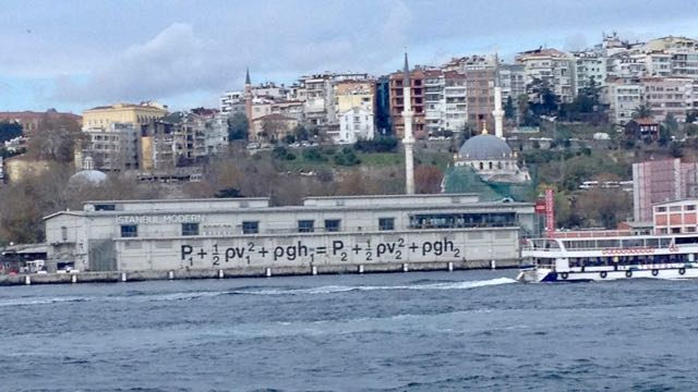
It is also valid for liquids
Pressure + Kinetic + Gravitational potential = Constant
(Pressure is an elastic potential)
Robots are coming
Google’s DeepMind predicts 3D shapes of proteins
“The ability to predict the shape that any protein will fold in to is a big deal. It has major implications for solving many 21st-century problems, impacting on health, ecology, the environment and basically fixing anything that involves living systems.
Liam McGuffin, Reading University, leader of the best UK group in the competition (and my co-author)
What, When and Where
What is the minimal speed?
plot(speed~time, data=coil)

When the coil has minimal speed?
plot(speed~time, data=coil)

How to find them in R?
min(coil$speed)
[1] -1.268
which.min(coil$speed)
[1] 26