November 29, 2018
Errata
Last class I made a mistake in one slide
I want to correct that mistake now

With experimental data from the big coil we found the linear model \[\text{n_marbles}=A+B\cdot \text{length}\] and we compared it with the formula from Hooke’s Law \[\text{force}=K\cdot(L-\text{length})\]
force is the weight of the marbles
Each marble has mass \(m\). The force points down, so \[-m g\cdot\text{n_marbles}=K\cdot(L-\text{length})\] which can be re-written as \[\text{n_marbles}=\underbrace{-\frac{K}{m g}\cdot L}_{A} + \underbrace{\frac{K}{m g}}_{B}\cdot\text{length} \]
CGS units
In this case it is easier to use centimeters, grams and seconds
Thus, force is measured in dyne, and length in cm
Looking at Hooke’s law \[\text{force}=K\cdot(L-\text{length})\] we can see that \(K\) is measured in dyne/cm
Finding \(K\)
Our model is \[\text{n_marbles}=\underbrace{-\frac{K}{m g}\cdot L}_{\texttt{coef(model)[1]}} + \underbrace{\frac{K}{m g}}_{\texttt{coef(model)[2]}}\cdot\text{length}\] therefore \[K=\texttt{coef(model)[2]}\cdot m\cdot g\]
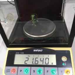
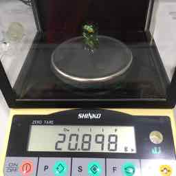
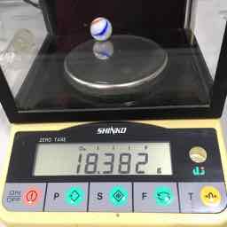
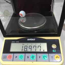
Marbles weight \(\approx 20\pm 1\) grams
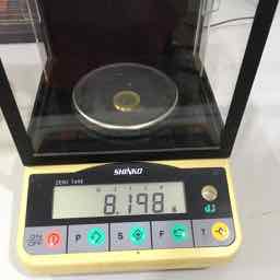
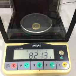
Calculating \(K\)
Taking the mass of marbles as 20gr, we calculate the elasticity constant as
coef(model)[2] * 20 * 9.8
length
  37.5
The units are dyne/cm.
The label length comes from coef(model)[2]
The number is the same as before. The units are correct this time
Calculating \(L\)
This is the same as last class. Since
\[\texttt{coef(model)[1]}=-\frac{K}{m g}L = -\texttt{coef(model)[1]}\cdot L \] we can calculate \(L\) as \[L=-\frac{\texttt{coef(model)[1]}}{\texttt{coef(model)[2]}} = 75.922\]
Logarithmic models
What is a logarithm?
We need very little math for our course: arithmetic, algebra, and logarithms
If \(x=p^m\) then \[\log_p(x) = m\]
If we use another base, for example \(q\), then \[\log_q(x) = m\cdot\log_q(p)\]
So if we use different bases, there is only a scale factor
The easiest one is natural logarithm
Other things about logarithms
- They only work with positive numbers. Not with 0
- If \(x=p\cdot q\) then \[\log(x)=\log(p)+\log(q)\]
- If \(\log(x)=m\) then \(x=\exp(m)\)
Linear models can be used in three cases
Basic linear model \[y=A+B\cdot x\] Exponential \[y=I\cdot R^x\qquad\log(y)=log(I)+log(R)\cdot x\] Power of \(x\) \[y=C\cdot x^E\qquad\log(y)=log(C)+E\cdot\log(x)\]
Which one to use?
The easiest way to decide is to draw several plots, placing log() in different places, and looking which one seems more like a straight line
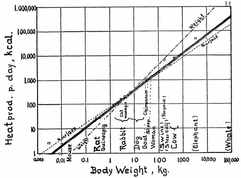
For example, let’s analyze data from Kleiber’s Law (Physiological Reviews 1947 27:4, 511-541)
The following data shows a summary. The complete table has 26 animals
Body size v/s metabolic rate
| animal | kg | kcal |
|---|---|---|
| Mouse | 0.021 | 3.6 |
| Rat | 0.282 | 28.1 |
| Guinea pig | 0.410 | 35.1 |
| Rabbit | 2.980 | 167.0 |
| Cat | 3.000 | 152.0 |
| Macaque | 4.200 | 207.0 |
| Dog | 6.600 | 288.0 |
| animal | kg | kcal |
|---|---|---|
| Goat | 36.0 | 800 |
| Chimpanzee | 38.0 | 1090 |
| Sheep ♂ | 46.4 | 1254 |
| Sheep ♀ | 46.8 | 1330 |
| Woman | 57.2 | 1368 |
| Cow | 300.0 | 4221 |
| Young cow | 482.0 | 7754 |
First plot: Linear
plot(kcal ~ kg, data=kleiber)

Second plot: semi-log
plot(log(kcal) ~ kg,
     data=kleiber)

Third plot: log-log
plot(log(kcal) ~ log(kg), data=kleiber)

Which one seems more “straight”?
The plot that seems more straight line is the log-log plot.
Therefore we need a log-log model.
A parenthesis
A comment about plots
Depending on the context, we may want to use different versions of semi-log and log-log plots
For understanding the data, we do
plot(log(kcal) ~ kg, data=kleiber)
For publishing in a paper, we do
plot(kcal ~ kg,
    data=kleiber, log="y")
Example
plot(log(kcal) ~ kg,
data=kleiber)

plot(kcal ~ kg,
data=kleiber, log="y")

Example
plot(log(kcal) ~ log(kg),
     data=kleiber)

plot(kcal ~ kg,
  data=kleiber, log="xy")

Which one seems more “straight”?
close parenthesis
The plot that seems more straight line is the log-log plot
Therefore we need a log-log model.
model <- lm(log(kcal) ~ log(kg), data=kleiber)
coef(model)
(Intercept)     log(kg)
      4.206       0.756
What is the interpretation of these coefficients?
If \[\log(kcal)=4.206 + 0.756\cdot \log(kg)\] then \[kcal=\exp(4.206) \cdot kg^{0.756}\]
Therefore:
- The average energy consumption of a 1kg animal is \(\exp(4.206) = 67.072\) kcal
- The energy consumption increases at a rate of \(0.756\) kcal/kg.
This is Kleiber’s Law
“An animal’s metabolic rate scales to the ¾ power of the animal’s mass”.
Google it
Using the model to predict
What can we do with the model?
Models are the essence of scientific research
They provide us with two important things
- An explanation for the observed patterns of nature
- A method to predict what will happen in the future
Predicting with the model
predict(model, newdata)
where newdata is a data frame with column names corresponding to the independent variables
If we omit newdata, the prediction uses the original data as newdata
predict(model) == predict(model, newdata=data)
Results
What is wrong here?
| animal | kg | kcal | predicted |
|---|---|---|---|
| Mouse | 0.021 | 3.6 | 1.28 |
| Rat | 0.282 | 28.1 | 3.25 |
| Guinea pig | 0.410 | 35.1 | 3.53 |
| Rabbit | 2.980 | 167.0 | 5.03 |
| Cat | 3.000 | 152.0 | 5.04 |
| Macaque | 4.200 | 207.0 | 5.29 |
| Dog | 6.600 | 288.0 | 5.63 |
| animal | kg | kcal | predicted |
|---|---|---|---|
| Goat | 36.0 | 800 | 6.92 |
| Chimpanzee | 38.0 | 1090 | 6.96 |
| Sheep ♂ | 46.4 | 1254 | 7.11 |
| Sheep ♀ | 46.8 | 1330 | 7.11 |
| Woman | 57.2 | 1368 | 7.26 |
| Cow | 300.0 | 4221 | 8.52 |
| Young cow | 482.0 | 7754 | 8.88 |
Undoing the logarithm
We want to predict the metabolic rate, depending on the weight
The independent variable is \(kg\), the dependent variable is \(kcal\)
But our model uses only \(\log(kg)\) and \(\log(kcal)\)
So we have to undo the logarithm, using \(\exp()\)
Correct formula for prediction
predicted_kcal <- exp(predict(model))
| animal | kg | kcal | predicted |
|---|---|---|---|
| Mouse | 0.021 | 3.6 | 3.62 |
| Rat | 0.282 | 28.1 | 25.76 |
| Guinea pig | 0.410 | 35.1 | 34.19 |
| Rabbit | 2.980 | 167.0 | 153.11 |
| Cat | 3.000 | 152.0 | 153.89 |
| Macaque | 4.200 | 207.0 | 198.46 |
| Dog | 6.600 | 288.0 | 279.29 |
| animal | kg | kcal | predicted |
|---|---|---|---|
| Goat | 36.0 | 800 | 1007 |
| Chimpanzee | 38.0 | 1090 | 1049 |
| Sheep ♂ | 46.4 | 1254 | 1220 |
| Sheep ♀ | 46.8 | 1330 | 1228 |
| Woman | 57.2 | 1368 | 1429 |
| Cow | 300.0 | 4221 | 5001 |
| Young cow | 482.0 | 7754 | 7157 |
Visually
plot(log(kcal) ~ log(kg), data=kleiber)
lines(predict(model) ~ log(kg), data=kleiber)
 ## Visually
plot(kcal ~ kg, data=kleiber, log="xy")
lines(exp(predict(model)) ~ kg, data=kleiber)

In the paper
Exponential growth in Science and Technology
Moore’s Law
A idea originated around 1970, by George Moore from Intel
The simple version of this law states that processor speeds will double every two years
More specifically, it says that the number of transistors on an affordable CPU would double every two years
(see paper)

Intel says
Real data: Number of transistors in chips v/s year
plot(count~Date, data=trans)

Semilog scale: Number of transistors v/s year
plot(log(count) ~ Date, data=trans)

Semi-log means exponential growth
we have straight line on the semi-log
That is, log(y) versus x \[\log(y)=log(I)+log(R)\cdot x\] In this case the original relation is \[y=I\cdot R^x\]
Model
model <- lm(log(count) ~ Date, data=trans)
exp(coef(model))
(Intercept)        Date
  7.83e-295    1.41e+00
Semi-log scale and model
plot(count ~ Date, data=trans, log="y")
lines(exp(predict(model)) ~ Date, data=trans)

Meaning
Every year processors grow by a factor of
exp(coef(model)[2])
Date
1.41
Same happens with DNA
Cost of sequencing human genome

What does this mean for you?
The Robots Are Coming
John Lanchester
- 1992 Russo-American moratorium on nuclear testing
- 1996 Computer simulations to design new weapons
- Needed more computing power than could be delivered by any existing machine
The Robots Are Coming
John Lanchester
- USA designed ASCI Red, the first supercomputer doing over one teraflop
- ‘flop’ is a floating point operation (multiplication) per second
- teraflop is \(10^{12}\) flops
- In 1997, ASCI Red did 1.8 teraflops
- The most powerful supercomputer in the world until about the end of 2000.
The Robots Are Coming
In his book, John Lanchester says
"I was playing on Red only yesterday – I wasn’t really, but I did have a go on a machine that can process 1.8 teraflops.
"This Red equivalent is called the PS3: it was launched by Sony in 2005 and went on sale in 2006.
The Robots Are Coming
"Red was [the size of] a tennis court, used as much electricity as 800 houses, and cost US$55 million. The PS3 fits under the TV, runs off a normal power socket, and you can buy one for £200.
"[In 10 years], a computer able to process 1.8 teraflops went from being something that could only be made by the world’s richest government […], to something a teenager could expect [as a gift].