November 26, 2018
Why?
Why are we here?
To become a Scientist
Someone who does Science
Science is not only making experiments
Science is the process of creating knowledge
We search for truth with the Scientific Method
Scientific Method
- We observe the nature and find patterns
- We create models that can explain the patterns
- We make experiments to test if the models are valid
This way we avoid fooling ourselves
Scientist look for the truth
- Does smoking causes cancer?
- Does eating sugar makes you fat?
- Does your cellphone produce brain cancer?
- Will an expensive medicine cure your sickness?
The society expect from us, the scientists, to answer these questions with the truth
Even in everyday jobs
Tomorrow you may work in a blood bank. Is the blood safe?
Or in a food factory. Is the food safe? Is it GMO?
Or in a University. Is this pharmaceutical company telling the truth?
Or you do a paternity test. Is this person the real father?
You are the Guardians of the Truth
Truth is essential for scientists
- Sometimes your experiments fail
- Sometimes you get a wrong result
- Sometimes your model is incomplete
- Most models are incomplete, and we are always updating them
You can be wrong, but you cannot lie
Some key parts of the Scientific Method
Models are tested with experiments
To be valid, experiments must be replicable
- That is, other people doing the same experiment must get the same result
There may be some variation between experiments
- You must declare what is your margin of error
- Every measurement has a margin of error
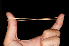
Coils and Rubber Bands
Coils
- Coils and rubber bands have a natural size
- If you apply a force to them, they expand
- What is the relation between the expansion and the force?
- We can put different weights and use gravity force
Results
| n_marbles | length | repetition |
|---|---|---|
| 0 | 78.00 | 1 |
| 1 | 82.61 | 1 |
| 2 | 85.85 | 1 |
| 3 | 90.26 | 1 |
| 4 | 95.05 | 1 |
| 0 | 79.21 | 2 |
| 2 | 85.55 | 2 |
| 3 | 90.06 | 2 |
| 4 | 94.35 | 2 |
| (some data o | mitted fr | om the table) |

Best-fit line
When data seems to be in a straight line, we can find that line
The best-fitting line is found using a linear model
model <- lm(n_marbles ~ length, data=rubber)
model
Call:
lm(formula = n_marbles ~ length, data = rubber)

Coefficients:
(Intercept)       length
   -14.5354       0.1915
What are the coefficients?
Remember that straight lines can be represented by the formula \[\text{n_marbles}=A+B\cdot \text{length}\] The coefficient \(A\) is the value where the line intercepts the vertical axis
The coefficient \(B\) is how much length goes up when n_marbles increases. This is called slope
In our case \(A\) and \(B\) are
(Intercept)      length
-14.5353768   0.1914521
Robert Hooke said it first
 Robert Hooke (1635–1703) was an English natural philosopher, architect and polymath.
In 1660, Hooke discovered the law of elasticity which describes the linear variation of tension with extension
“The extension is proportional to the force”
Robert Hooke
![]() Natural philosophy was the study of nature and the physical universe that was dominant before the development of modern science
Natural philosophy was the study of nature and the physical universe that was dominant before the development of modern science
Polymath (from Greek “having learned much”) is a person whose expertise spans a significant number of different subject areas
Biologist. Hooke used the microscope and was the fists to use the term cell for describing biological organisms.
How do we model a coil?
The essence of the coil is:
- It has a natural length \(L\)
- If we change the length by \(x\), it pulls with a force \[\mathrm{force}(x)= K \cdot (L-x)\]
Physical interpretation of the linear model
The formula from Hooke’s Law is \[\text{force}=K\cdot(L-\text{length})\] Since force is the weight of the marbles, we can write \[-m g\cdot\text{n_marbles}=K\cdot(L-\text{length})\] which can be re-written as \[\text{n_marbles}=\frac{K}{m g}\cdot\text{length} - \frac{K}{m g}\cdot L\]
Physical interpretation of coef(model)
Comparing the formulas we can see that \[\texttt{coef(model)[2]}=\frac{K}{m g}\quad\text{thus}\quad K=\texttt{coef(model)[2]}\cdot m\cdot g\] If the mass of each ball is 20gr, we can find \(K\) as
coef(model)[2] * 20 * 9.8
  length
37.52461
This is the elasticity constant. The units are dyne/cm
Natural length of the coil
We also see that \[\texttt{coef(model)[1]}=-\frac{K}{m g}L = -\texttt{coef(model)[1]}\cdot L \] Therefore \[L=-\frac{\texttt{coef(model)[1]}}{\texttt{coef(model)[2]}}\]
Natural length of the coil
When there are no balls, the natural length of the coil is \(L\)
This value is hard to measure directly
But, using the formula from the regression, we have
-coef(model)[1]/coef(model)[2]
(Intercept)
   75.92175
Replicability
Can we replicate your experiments?
I cleaned up all the files
There are two that I could not recover
The rest are either “coins” or “marbles”
Coins
| A | B | K | L |
|---|---|---|---|
| -32.640000 | 4.3200000 | 347.15520 | 7.555556 |
| -22.631714 | 3.1202046 | 250.73964 | 7.253279 |
| -14.514493 | 1.8840580 | 151.40290 | 7.703846 |
| -13.590202 | 1.9517885 | 156.84572 | 6.962948 |
| -12.349076 | 1.6837782 | 135.30842 | 7.334146 |
| -11.000000 | 1.2857143 | 103.32000 | 8.555556 |
| -9.621145 | 2.9074890 | 233.64581 | 3.309091 |
| -8.728814 | 1.1525424 | 92.61831 | 7.573529 |
| -5.058176 | 0.5554427 | 44.63538 | 9.106567 |
Plot Coins

Marbles
| A | B | K | L |
|---|---|---|---|
| -18.305520 | 2.2721438 | 445.34018 | 8.056497 |
| -11.285714 | 1.4285714 | 280.00000 | 7.900000 |
| -10.039956 | 1.2005156 | 235.30105 | 8.363037 |
| -9.366083 | 1.9008064 | 372.55805 | 4.927426 |
| -5.048315 | 0.5550562 | 108.79101 | 9.095142 |
| -5.048315 | 0.5550562 | 108.79101 | 9.095142 |
| -4.986521 | 0.5518820 | 108.16887 | 9.035484 |
| -3.278303 | 0.0643182 | 12.60636 | 50.970104 |
Plot Marbles

Exponential growth
How cells grow
We want to know the number of cells every day, which we represent with the vector ncell
Each element of the vector is the number of cells in day t
We start with an initial number of cells, that we call initial
Each day, the number of cells increases by a factor rate
Recurrence
The number of cells on day t is ncell[t]
Each day the number of cell is multiplied by rate
Therefore ncell[t] = rate * ncell[t-1]
This is a recursive formula
Can you write an explicit formula? (non-recursive)
Formula
The solution of the recurrence is
ncell[t] = initial * rate^t
In R we can do this easily when t is a vector
t <- seq(from=start, to=end, by=step)
ncell <- initial * rate ^ t
Graphic
t <- 1:20
initial <- 20
rate <- 2
ncells <- initial * rate^t
ncells
 [1]       40       80      160      320      640     1280     2560     5120    10240
[10]    20480    40960    81920   163840   327680   655360  1310720  2621440  5242880
[19] 10485760 20971520
Graphic
plot(t, ncells)
 We cannot see what happens when values are small
Logarithmic scale (“semi-log”)
plot(log(ncells) ~ t)
 We can see better using a logarithmic vertical scale
Why?
We have many cases when the values increase (or decrease) with a factor
For example, the cost of DNA sequencing
In general if the relation is \[y = I\cdot R^x\] we can get a better picture applying logarithms \[\log(y) = \log(I\cdot R^x) = \log(I) + x \log(R)\]
Other cases
Sometimes the formula is different. For example the area of a circle is \[a=\pi r^2\] and the volume of a sphere is \[v=\frac{4}{3}\pi r^3\]
General case
In general you can have \[y= A x^B\] then, using logarithms, you have \[\log(y)=\log(A x^B)=\log(A) + B\log(x)\] Now we need also \(\log(x)\)
Log-log scale
par(mfrow=c(1,2))
plot(t, 2*t^3)
plot(t, 2*t^3, log="xy")

Using log in linear models
When the logarithmic scale shows a straight line, we can use a linear model
We have to be careful to use log and exp in the correct place
Example
Let’s consider this case
example <- data.frame(t, vol=2*t^3)
head(example)
  t vol
1 1   2
2 2  16
3 3  54
4 4 128
5 5 250
6 6 432
Plot Using logarithm
par(mfrow=c(1,2))
plot(vol~t, data=example)
plot(log(vol)~t, data=example)
 Log-log scale looks straight
Model
model <- lm(log(vol)~log(t), data=example)
model
Call:
lm(formula = log(vol) ~ log(t), data = example)

Coefficients:
(Intercept)       log(t)
     0.6931       3.0000
exp(coef(model)[1])
(Intercept)
          2