In general, when the Scoring matrix changes, then the optimal alignment also changes
For example, if mismatches are expensive then the method may use more gaps
But if we multiply every score by a positive constant, then the alignment does not change
November 27, 2018
In general, when the Scoring matrix changes, then the optimal alignment also changes
For example, if mismatches are expensive then the method may use more gaps
But if we multiply every score by a positive constant, then the alignment does not change
For example, if we align DNA with
every decision will be the same as when the score is
The alignment does not change if the scoring matrix \(S\) is replaced by another matrix \(\lambda S\)
(this is valid for any positive number \(\lambda\))
What is the best \(\lambda\)?
To answer that question we have to understand how the Scoring matrices are built
As we have seen, scoring matrices are built based on a previous alignment
Margaret Dayhoff took 71 families of closely related proteins
Inside each family all sequences had at least 85% of identical residues
She built the alignments manually, and calculated the frequency of mutation for each pair of residues
The same procedure was done by Henikoff and Henikoff, but using only the conserved domains of proteins
In both cases, they observed each residue
and they calculated the proportion \(r_{ab}\) of residues \(a\) aligned to \(b\)
Assuming that this is a good alignment
TAATACCGCATAATAATCAGTTTTCACATGGAGACTGATTTAAAGGAGTAATCCGCTT
TAATACCGCATAACATTAGTATTTCACATGAAGTACTAATTAAAGGAGTAATCCGCTT
   b
a       A     C     G     T
  A 29.31  1.72  1.72  3.45
  C  1.72 13.79  0.00  1.72
  G  1.72  0.00 12.07  1.72
  T  3.45  1.72  1.72 24.14
These observed proportions can be seen as an estimation of the probability of aligning two residues when they have a common ancestor
We want to compare this against the probability of aligning two unrelated residues. We will compare two hypothesis
\(H_0\): there is no common ancestor
\(H_1\): there is a common ancestor
As we said, when there is a common ancestor, we have \[\Pr(a,b|H_1) = r_{ab}\] In the other case, if there is no common ancestor, then \(a\) and \(b\) are independent, thus \[\Pr(a, b|H_0) = \Pr(a|H_0)\Pr(b|H_0)=p_{a}p_{b}\] where \(p_a\) is simply the proportion of residue \(a\) in all the sequences
(independent probabilities means that we can multiply them)
To compare these two probabilities we can take their ratio \[\frac{\Pr(a,b|H_1)}{\Pr(a, b|H_0)}=\frac{r_{ab}}{p_a p_b}\] If this value is greater than 1, then \(H_1\) is more plausible than \(H_0\)
It can be proved that this value is proportional to \[\Pr(H_1| a\text{ aligns with }b)\] which is really what we are looking for
In practice it is much easier to work with the logarithm of it \[\log\frac{\Pr(a,b|H_1)}{\Pr(a, b|H_0)}=\log \frac{r_{ab}}{p_a p_b}\] This number is positive when \(H_1\) is more plausible than \(H_0\), and negative otherwise
We want to extend this to the complete sequences \(q\) and \(s\)
Assuming that each residue is independent, we have \[\Pr(q,s|H_1)=\Pr(q_1,s_1|H_1)\cdot\Pr(q_2,s_2|H_1)\cdots\Pr(q_n,s_n|H_1)\] The same formula works for \(H_0\), so \[\frac{\Pr(q,s|H_1)}{\Pr(q,s|H_0)}=\frac{\Pr(q_1,s_1|H_1)}{\Pr(q_1,s_1|H_0)}\cdot\frac{\Pr(q_2,s_2|H_1)}{\Pr(q_2,s_2|H_0)}\cdots\frac{\Pr(q_n,s_n|H_1)}{\Pr(q_n,s_n|H_0)}\]
(here we assume that \(q\) and \(s\) may contain gaps so they have equal length \(n\))
\[\log\frac{\Pr(q,s|H_1)}{\Pr(q,s|H_0)}=\log\frac{\Pr(q_1,s_1|H_1)}{\Pr(q_1,s_1|H_0)}+\log\frac{\Pr(q_2,s_2|H_1)}{\Pr(q_2,s_2|H_0)}+\cdots+\log\frac{\Pr(q_n,s_n|H_1)}{\Pr(q_n,s_n|H_0)}\] That is \[\log\frac{\Pr(q,s|H_1)}{\Pr(q,s|H_0)}=\sum_{i=1}^n\log\frac{\Pr(q_i, s_i|H_1)}{\Pr(q_i, s_i|H_0)} = \sum_{i=1}^n \log \frac{r_{q_i s_i}}{p_{q_i}p_{s_i}}\] This sum is a score of the alignment!
Let’s assume that we have an alignment of \(q\) and \(s\), that is, we have gaps inside \(q\) and \(s\) so they have the same length \(n\)
If we have a scoring matrix \(S\) We can find its score as the sum \[\sum_{i=1}^n S[q_i, s_i]\] Comparing this with the previous slide we find that \[\log \frac{r_{q_i s_i}}{p_{q_i}p_{s_i}}\] can be used as a score.
Remember that the score can be multiplied by \(\lambda\) without any effect on the alignment.
Simplifying, we can say \[\lambda S[a,b]=\log \frac{r_{ab}}{p_{a}p_{b}}\]
According to WikiPedia, they used the formula \[\lambda S[a,b]=\text{round}\left(2\cdot\log_2 \frac{r_{ab}}{p_{a}p_{b}}\right)\] that is, rounded to the nearest integer
Computers work faster with integer numbers, so PAM and BLOSUM drop the decimals
The factor 2 is used to get more information before rounding
We have seen the process from probabilities to score matrix
In the other way,
Let’s say that the score for match is 1, and we will try different values for mismatch, like -1, -2,…, -5
In this case we have 4 letters, that we assume have the same probability. Thus \[p_a = \frac{1}{4}\quad\text{ for all }a\in \{A,C,G,T\}\]
To find \(r_{ab}\) we need to find \(\lambda\), because \[\lambda S[a,b]=\log \frac{r_{ab}}{p_{a}p_{b}}\] and therefore \[r_{ab}= p_a p_b \exp(\lambda S[a,b])\]
Notice that so far we did not say what was the logarithm’s base
Here we chose natural logarithms, but in theory it can be any base
In this case we also know that \[\sum_{a,b} r_{ab}=1\] therefore \[\sum_{ab} p_a p_b \exp(\lambda S[a,b]) = 1\] This condition allows us to find \(\lambda\)
Let’s consider the function \[f(x)=\sum_{a,b}p_a\, p_b\, \exp(x\, S_{a,b})\] so \(f(\lambda)=1\). When \(x=0\) we have \[f(0)=\sum_{a,b}p_a\, p_b\, \exp(0) = \sum_{a}p_a\, \sum_{b}p_b = 1\] because \(p_a\) and \(p_b\) are probabilities. But we want \(\lambda>0\)
It can be proved that always \(f(x)\) looks like this: 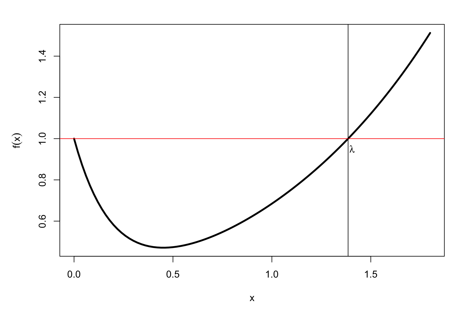
It is easy to find \(\lambda\) with a computer 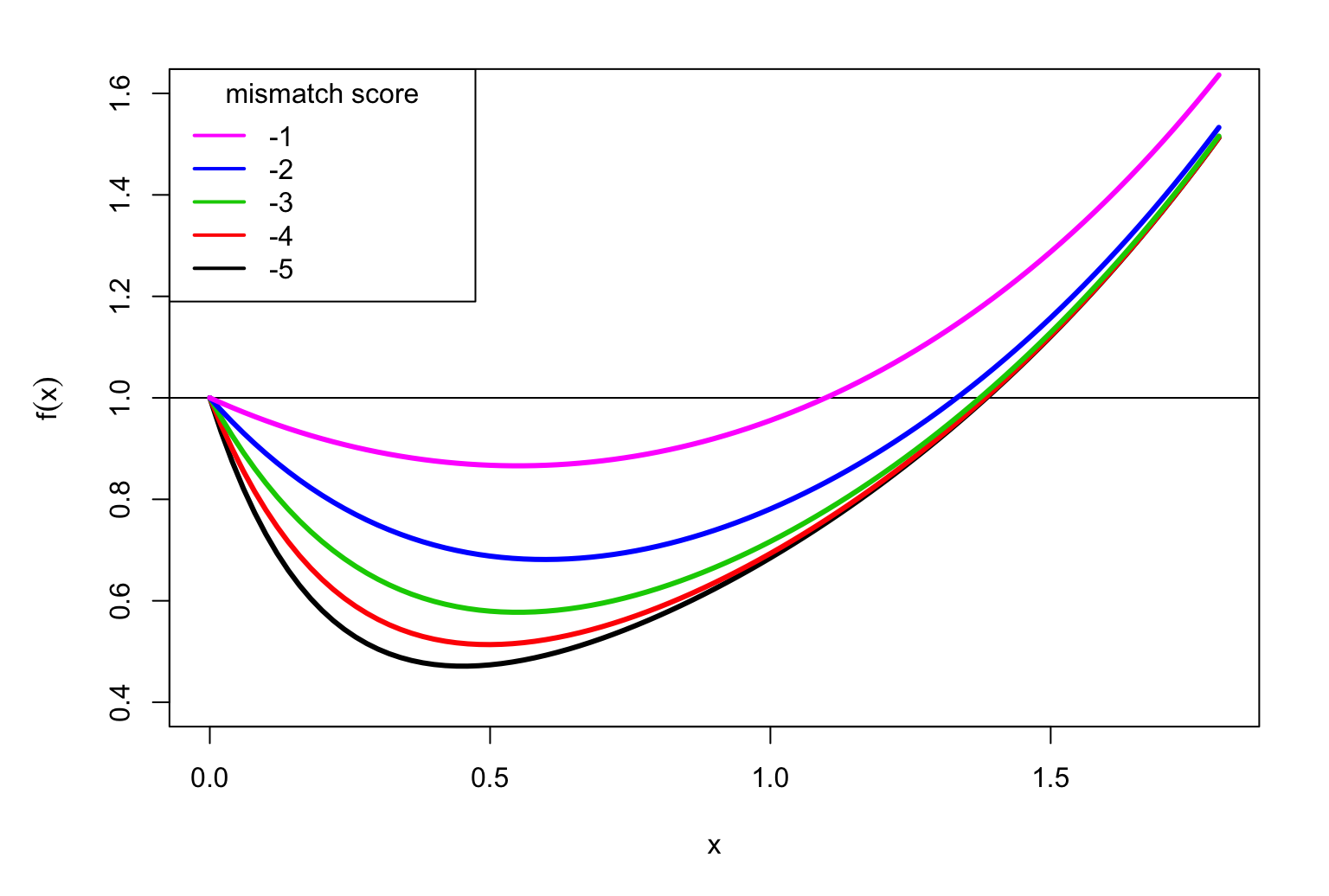
For match = 1 and mismatch = -2 we have \(\lambda=1.333\)
The \(r_{ab}\) probability matrix is
       A      C      T      G
A 23.691  0.435  0.435  0.435
C  0.435 23.691  0.435  0.435
T  0.435  0.435 23.691  0.435
G  0.435  0.435  0.435 23.691
For match = 1 and mismatch = -5 we have \(\lambda=1.385\)
The \(r_{ab}\) probability matrix is
         A        C        T        G
A 24.97400  0.00614  0.00614  0.00614
C  0.00614 24.97400  0.00614  0.00614
T  0.00614  0.00614 24.97400  0.00614
G  0.00614  0.00614  0.00614 24.97400
Once we know \(\lambda\) we can determine the probabilities of mutation \[q_{a,b}= p_a\, p_b\, \exp(\lambda S_{a,b})\] Now we can, for example, determine the average identity between two aligned sequences \[\sum_a p_a\, q_{a,a}\] that is, the average probability that a residue is conserved
| match | mismatch | lambda | Avg.ident |
|---|---|---|---|
| 1 | -1 | 1.098 | 75 |
| 1 | -2 | 1.333 | 94.8 |
| 1 | -3 | 1.375 | 98.8 |
| 1 | -4 | 1.383 | 99.7 |
| 1 | -5 | 1.385 | 99.9 |
| 2 | -3 | 0.6333 | 47.1 |
| 4 | -5 | 0.3013 | 33.8 |