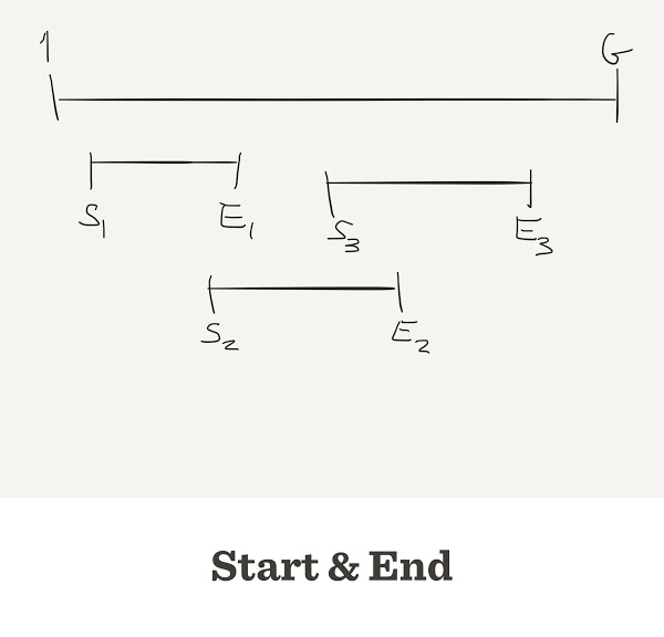
The number of contigs depends on

• Genome length: G
• Length of reads: L
• Number of reads: N

In general L can be different for each read. In this simulation we will assume all reads have the same length

Exercise: Find the real values of L in our reads

sim_sequencing <- function(N, L, G) {
  start <- sample.int(G, size=N)
  end <- start + L
  depth <- rep(0, G)
  for(i in 1:N) {
    read_pos <- start[i]:min(end[i], G)
    depth[read_pos] <- depth[read_pos] + 1
  }
  return(depth)
}

Depth is a property of each position in the genome

Depth average is also known as coverage

Coverage can be calculated before sequencing

get_coverage <- function(N, L, G) {
    return(N*L/G)
}

This is the percentage of the genome that we can see with our reads

We can only know coverage breadth after we assembly

Moreover, we can ask for coverage breadth with a minimum depth

get_breadth <- function(depth, G, MIN=0) {
    return(sum(depth>MIN)/G)
}

The question we want to answer is

How many reads we need to see all the genome with a minimum depth?

How would you answer that question?

So far we have assumed that we know the exact position of the read in the geome

That is never true

What classic assemblers do is to find when the end of one read is equal to the start of another read

That is called overlap

overlap <- rep(NA, N-1)
for(i in 1:(N-1)) {
  overlap[i] <- end[i] - start[i+1]
}

overlap_sizes <- function(N, L, G) {
  start <- sample.int(G, N) # shotgun
  start <- sort(start) # This is important
  end <- start + L
  overlap <- rep(NA, N-1)
  for(i in 1:(N-1)) {
    overlap[i] <- end[i] - start[i+1]
  }
  return(overlap)
}

Exercise: can we avoid the for() loop?

overlap_sizes <- function(N, L, G) {
  start <- sample.int(G, N) # shotgun
  start <- sort(start) # This is important
  end <- start + L
  overlap <- end[-N] - start[-1]
  return(overlap)
}

We only see overlaps over a threshold thr

The best thr has to be big enough to guarantee that the reads do not overlap by chance

Bigger values of thr reduce the probability of “overlap by chance”

A group of contiguous sequences is called Contig

The goal of the assembly process is to find one contig.

The sequence of this contig will be the genome

Most of times we do get several contigs

num_contigs <- function(N, L, G, thr) {
  num_gaps <- sum(overlap_sizes(N, L, G) < thr)
  return(num_gaps)
}

num.reads <- seq(from=10, to=5E4, by=2E3)
n.contigs <-  rep(NA, length(num.reads))
for(k in 1:length(num.reads)) {
    n.contigs[k] <- num_contigs(N=num.reads[k], L=100,
                                G=1e6, thr=20)
}

plot(n.contigs ~ num.reads, type="b")

num.reads <- seq(from=10, to=5E4, by=2E3)
n.contigs <- sapply(num.reads, num_contigs, L=100,
                    G=1e6, thr=20)

plot(n.contigs ~ num.reads, type="b")

With this simulation we can also calculate the length of each contig.

contig_len

[1]  149 1377  401 1363 1450  265 2001  351

sum(contig_len)

[1] 7357

Given a set of contigs, the N50 is defined as the sequence length of the shortest contig at 50% of the total genome length

We sort the contigs from largest to smallest

sort(contig_len, decreasing = TRUE)

[1] 2001 1450 1377 1363  401  351  265  149

Prepare a presentation about NGS

• Each person chooses one different method
• Find the “standard protocol”
• Find the typical fragment size, read size, number of reads
• Typical error rates
• Time, cost (Turkey or abroad)

• Indiana University Bloomington, “Introduction to Bioinformatics”, Lecture by Yuzhen Ye

• Université Lyon I, Network Algorithms for Molecular Biology lesson on “Introduction to (de novo) assembly”, by Blerina Sinaimeri

• MIT, “Foundations of Computational Systems Biology”, Lecture by David K. Gifford