Abstraction: forget details to make it generic
Formalization: avoid ambiguity and logic errors
Solution: use a computer or ask a friend
Interpret: this is the biology
23 September 2016
Steps
A simple model
choosing a representative
Choosing a representative
- Summarizing a set of observations with a single number
- the best “representative” is the one that minimizes the error
- the way we measure error determines which “representative” we choose
- the mean error measures the quality of the “representative”
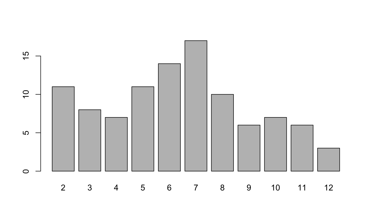
We get values from an experiment
2, 9, 6, 2, 5, 10, 4, 6, 8, 7, 11, 7, 6, 7, 8, 4, 7, 4, 2, 8, 3, 5, 7, 3, 7, 6, 7, 2, 4, 6, 5, 6, 12, 8, 6, 5, 6, 8, 3, 2, 7, 7, 6, 8, 9, 8, 11, 2, 6, 3, 11, 11, 5, 9, 7, 5, 8, 6, 11, 5, 7, 4, 5, 7, 3, 2, 10, 10, 10, 3, 3, 8, 7, 10, 10, 2, 2, 6, 7, 6, 4, 4, 9, 11, 12, 5, 2, 9, 2, 5, 10, 12, 7, 8, 6, 7, 3, 9, 7 and 5
Summaries: frequency table, barplot
| 2 | 3 | 4 | 5 | 6 | 7 | 8 | 9 | 10 | 11 | 12 |
|---|---|---|---|---|---|---|---|---|---|---|
| 11 | 8 | 7 | 11 | 14 | 17 | 10 | 6 | 7 | 6 | 3 |
Abstraction (a.k.a. generalization)
- We have a vector \(\mathbf{y}=(y_1,\ldots, y_n)\) with \(n\) observations, each one with value \(y_i\) for \(i\) taking values between 1 and \(n\)
- We want to represent this set by a single number \(\beta\). The model is \[\mathbf{y} = \beta + \mathbf{e}\] which is a short version of all the equations \[y_i = \beta + e_i\quad\mathrm{for}\quad i=1,\ldots,n\]
Representing \(\mathbf{y}\) with a single number
The model is \[\mathbf{y} = \beta + \mathbf{e}\]
- Here \(\mathbf{y}\) is your data
- We are “free” to chose \(\beta\)
- Each selection of \(\beta\) has different error \(\mathbf{e}\)
Which one is the best \(\beta\)?
How big is the error?
Several ways to define “error”
Mean absolute error \[\mathrm{MAE}(\beta, \mathbf{y})=\frac{1}{n}\sum_i |y_i-\beta|\]
Mean square error \[\mathrm{MSE}(\beta, \mathbf{y})=\frac{1}{n}\sum_i (y_i-\beta)^2\]
Mean absolute error
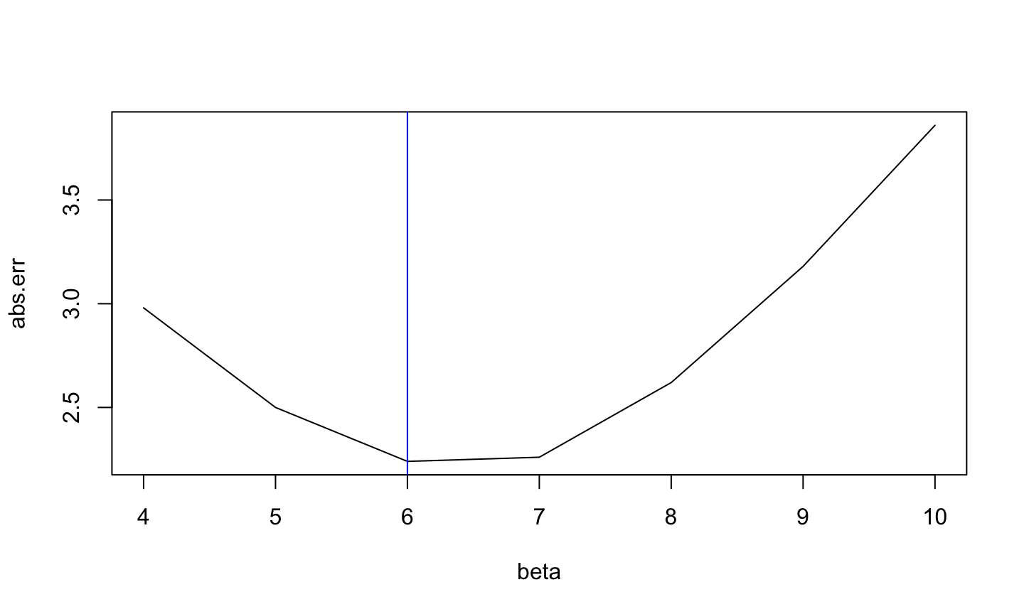
\[\beta^* = 6\]
Homework
Show that the median of \(\mathbf{y}\) is a minimum of the mean absolute error
Mean square error
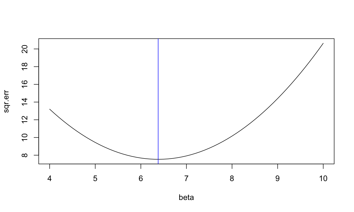
\[\beta^* = 6.38\]
Minimizing MSE
The error is \[\mathrm{MSE}(\beta, \mathbf{y})=\frac{1}{n}\sum_i (y_i-\beta)^2\]
To find the minimal value we can take the derivative of \(MSE\) with respect to \(\beta\)
\[\frac{d}{d\beta} \mathrm{MSE}(\beta, \mathbf{y})= \frac{2}{n}\sum_i (y_i - \beta)\]
The minimal values of functions are located where the derivative is zero
Minimizing MSE
Now we find the value of \(\beta\) that makes the derivative equal to zero.
\[\frac{d}{d\beta} \mathrm{MSE}(\beta, \mathbf{y})= \frac{2}{n}\sum_i (y_i - \beta)\]
Making this last formula equal to zero and solving for \(\beta\) we found that the best one is
\[\beta^* = \frac{1}{n} \sum_i y_i = \bar{\mathbf{y}}\]
Is this a good representative?
If \(\bar{\mathbf{y}}\) is the best representative, the error is
\[\mathrm{MSE}(\bar{\mathbf{y}}, \mathbf{y})=\frac{1}{n}\sum_i (y_i-\bar{\mathbf{y}})^2\]
This is sometimes called variance of the sample. We write then
\[\mathrm{S}_n(\mathbf{y})=\frac{1}{n}\sum_i (y_i-\bar{\mathbf{y}})^2\]
The order of \(\mathbf{y}\) is irrelevant
2, 2, 2, 2, 2, 2, 2, 2, 2, 2, 2, 3, 3, 3, 3, 3, 3, 3, 3, 4, 4, 4, 4, 4, 4, 4, 5, 5, 5, 5, 5, 5, 5, 5, 5, 5, 5, 6, 6, 6, 6, 6, 6, 6, 6, 6, 6, 6, 6, 6, 6, 7, 7, 7, 7, 7, 7, 7, 7, 7, 7, 7, 7, 7, 7, 7, 7, 7, 8, 8, 8, 8, 8, 8, 8, 8, 8, 8, 9, 9, 9, 9, 9, 9, 10, 10, 10, 10, 10, 10, 10, 11, 11, 11, 11, 11, 11, 12, 12 and 12
Each \(y_i\) appears \(N(y_i)\) times, given by the table
| 2 | 3 | 4 | 5 | 6 | 7 | 8 | 9 | 10 | 11 | 12 |
|---|---|---|---|---|---|---|---|---|---|---|
| 11 | 8 | 7 | 11 | 14 | 17 | 10 | 6 | 7 | 6 | 3 |
Alternative formula
With \(N(y_i)\) given by the table, we have
\[\bar{\mathbf{y}} = \frac{1}{n} \sum_i y_i = \sum_y y\cdot \frac{N(y)}{n} = \sum_y y \cdot p(y)\] \[\mathrm{MSE}(\bar{y}, \mathbf{y})=\frac{1}{n}\sum_i (y_i-\bar{\mathbf{y}})^2 =\sum_y (y-\bar{\mathbf{y}})^2\cdot p(y)\]
The empirical frequency \(p(y)=N(y)/n\) contains all the information of \(\mathbf{y}\)
Models with more variables
Linear model
Now we have a second vector \(\mathbf{x}\)
The new model is \[{y}_i = \beta_0 + \beta_1{x}_i + {e}_i\] for \(i=1,\ldots,n\). All these equations can be written in one as \[\mathbf{y} = \beta_0\mathbf{1} + \beta_1\mathbf{x} + \mathbf{e}\]
Mean square error
Now we want to minimize \[\mathrm{MSE}(\begin{pmatrix}\beta_0\\ \beta_1\end{pmatrix}, \mathbf{y}, \mathbf{x}) = \frac{1}{n}\sum_i (y_i-\beta_0 - \beta_1{x}_i)^2\] which can also be written as \[\frac{1}{n}\sum_i e_i^2\] Indeed, we are minimizing the square of errors (like before)
Geometrical interpretation

Since ancient times it is known that \(a^2+b^2=c^2\)
- The sum of the squares is the square of the diagonal
Using this idea we see that \[\sum_i e_i^2 = \mathrm{length}(\mathbf{e})^2\]
So we want to minimize the lenght of vector \(\mathbf{e}\).
Minimizing \(\mathbf{e}\)rrors
- The vectors \(\mathbf{y}\), \(\mathbf{x}\) and \(\mathbf{e}\) have dimension \(n\)
- But the vectors \(\beta_0\mathbf{1} + \beta_1\mathbf{x}\) have only 2 degrees of freedom
- All these vectors lie in a plane of dimension 2
We want to find the “good” \(\beta_0\) and \(\beta_1\) that minimize the length of \(\mathbf{e}\)
Good values and right angles

- The “smallest” \(\mathbf{e}\) is the one perpendicular to the plane defined by \(\mathbf{1}\) and \(\mathbf{x}\)
- In particular
- The best \(\mathbf{e}\) is perpendicular to \(\mathbf{1}\)
- The best \(\mathbf{e}\) is perpendicular to \(\mathbf{x}\)
Dot product
linear algebra to the rescue
Ancient knowledge again:
The vector \(\mathbf{e}\) is perpendicular to \(\mathbf{x}\) if and only if
\[\mathbf{x}^T\mathbf{e}=0\]
In the same way, \(\mathbf{e}\) is perpendicular to \(\mathbf{1}\) if \[\mathbf{1}^T\mathbf{e}=0\]
Seeing the big picture
We can see the big picture if we use matrices: \[\begin{pmatrix}1 & x_1\\ \vdots & \vdots \\1 & x_n\end{pmatrix}= \begin{pmatrix}\mathbf{1} & \mathbf{x}\end{pmatrix}=\mathbf{A}\] \[\begin{pmatrix}\beta_0\\ \beta_1\end{pmatrix}=\mathbf{b}\] then the smallest \(\mathbf{e}\) obeys \[ \mathbf{A}^T \mathbf{e} = 0\]
Finding beta
The model was \[\mathbf{y} = \mathbf{Ab} + \mathbf{e}\] so the error is \[\mathbf{e} = \mathbf{y} - \mathbf{Ab}\] Multiplying by \(\mathbf{A}^T\) we have \[\mathbf{A}^T \mathbf{e} = \mathbf{A}^T \mathbf{y} - \mathbf{A}^T \mathbf{Ab}\]
Finding beta
To have \(\mathbf{A}^T \mathbf{e} = 0\) we need to make \[\mathbf{A}^T \mathbf{y} = \mathbf{A}^T \mathbf{Ab}^*\] We write \(\mathbf{b}^*\) because these are the “good” \(\beta_0^*\) and \(\beta_1^*\)
Now, if \(\mathbf{A}^T \mathbf{A}\) is “well behavied”, \[\mathbf{b}^* = (\mathbf{A}^T \mathbf{A})^{-1}\mathbf{A}^T \mathbf{y}\]
Mean Square Error
Replacing \(\mathbf{b}^* = (\mathbf{A}^T \mathbf{A})^{-1}\mathbf{A}^T \mathbf{y}\) in the formula of error \[\mathbf{e} = \mathbf{y} - \mathbf{Ab}\] we have \[\mathbf{e}^* = (\mathbf{I} - \mathbf{A}(\mathbf{A}^T \mathbf{A})^{-1}\mathbf{A}^T )\mathbf{y}\] (no surprise, simple substitution)
What happens to the mean square error \(\mathrm{MSE}(\mathbf{b}^*,\mathbf{y}, \mathbf{x})=\frac{1}{n}\sum_i e_i^2\)?
Mean Square Error
\[\begin{aligned} \mathrm{MSE}(\mathbf{b}^*,\mathbf{y}, \mathbf{x})&=\frac{1}{n}\sum_i e_i^2=\frac{1}{n}\mathbf{e}^T\mathbf{e}\\ &=\frac{1}{n}\mathbf{y}^T (\mathbf{I} - \mathbf{A}(\mathbf{A}^T \mathbf{A})^{-1}\mathbf{A}^T)^T(\mathbf{I} - \mathbf{A}(\mathbf{A}^T \mathbf{A})^{-1}\mathbf{A}^T) \mathbf{y}\\ &=\frac{1}{n}\mathbf{y}^T (\mathbf{I} - \mathbf{A}(\mathbf{A}^T \mathbf{A})^{-1}\mathbf{A}^T) \mathbf{y}\end{aligned}\] (do the algebra and see that many things vanish)
So the Mean Square Error depends on \(\mathbf{y}\) and \(\mathbf{A}\), which depends on \(\mathbf{x}\). Choose them carefully
Generalization
All the argument is valid if \(\mathbf{A}\) has any number of columns
- that is, any number of independent variables
- at least 1
- at most \(n\)
One variable case
mean
If \(\mathbf{A} =\mathbf{1}\) (no independent variable), then \[\begin{aligned} \mathbf{b}^* &= (\mathbf{A}^T \mathbf{A})^{-1}\mathbf{A}^T \mathbf{y}\\ \mathbf{b}^* &= (\mathbf{1}^T \mathbf{1})^{-1}\mathbf{1}^T \mathbf{y}\\ \mathbf{b}^* &=\frac{1}{n}\sum{y}_i \end{aligned}\] just as before
One variable case
mean square error
\[\begin{aligned} \frac{1}{n}\mathbf{e}^T\mathbf{e} &= \frac{1}{n}\mathbf{y}^T (\mathbf{I} - \mathbf{A}(\mathbf{A}^T \mathbf{A})^{-1}\mathbf{A}^T) \mathbf{y}\\ &= \frac{1}{n}\mathbf{y}^T (\mathbf{I} - \mathbf{1}(\mathbf{1}^T \mathbf{1})^{-1}\mathbf{1}^T) \mathbf{y}\\ &= \frac{1}{n}\mathbf{y}^T \mathbf{y} - \frac{1}{n}\mathbf{y}^T\mathbf{1}(n)^{-1}\mathbf{1}^T \mathbf{y}\\ &=\frac{1}{n}\sum{y}_i^2 - (\frac{1}{n}\sum{y}_i)^2 \end{aligned}\] just as before
“Well behavior”
The only condition to have a solution is \[\mathbf{A}^T \mathbf{A}\] has an inverse. This is equivalent to
All columns of \(\mathbf{A}\) are linearly independent