Welcome back
to “Computing for Molecular Biology 1”
We learned how todo this
 How did we do that?
Exploring all data
plot(birth)

Numeric v/s Numeric
plot(head ~ weight, data=birth)

Numeric v/s Factor
plot(weight ~ sex, data=birth)

Boxplot
Plotting a numeric value depending on a factor results in a boxplot
It is a graphical version of summary().
- The center is the median
- The box is between the first and third quartil (50% of cases)
- The wiskers extend a prediction of 95% of cases
- Points are outliers
Nicer boxplot
plot(weight ~ sex, data=birth, boxwex=0.2, notch=TRUE, col="grey")

Factor v/s Factor
birth$apgar5 <- as.factor(birth$apgar5)
plot(sex ~ apgar5, data=birth)

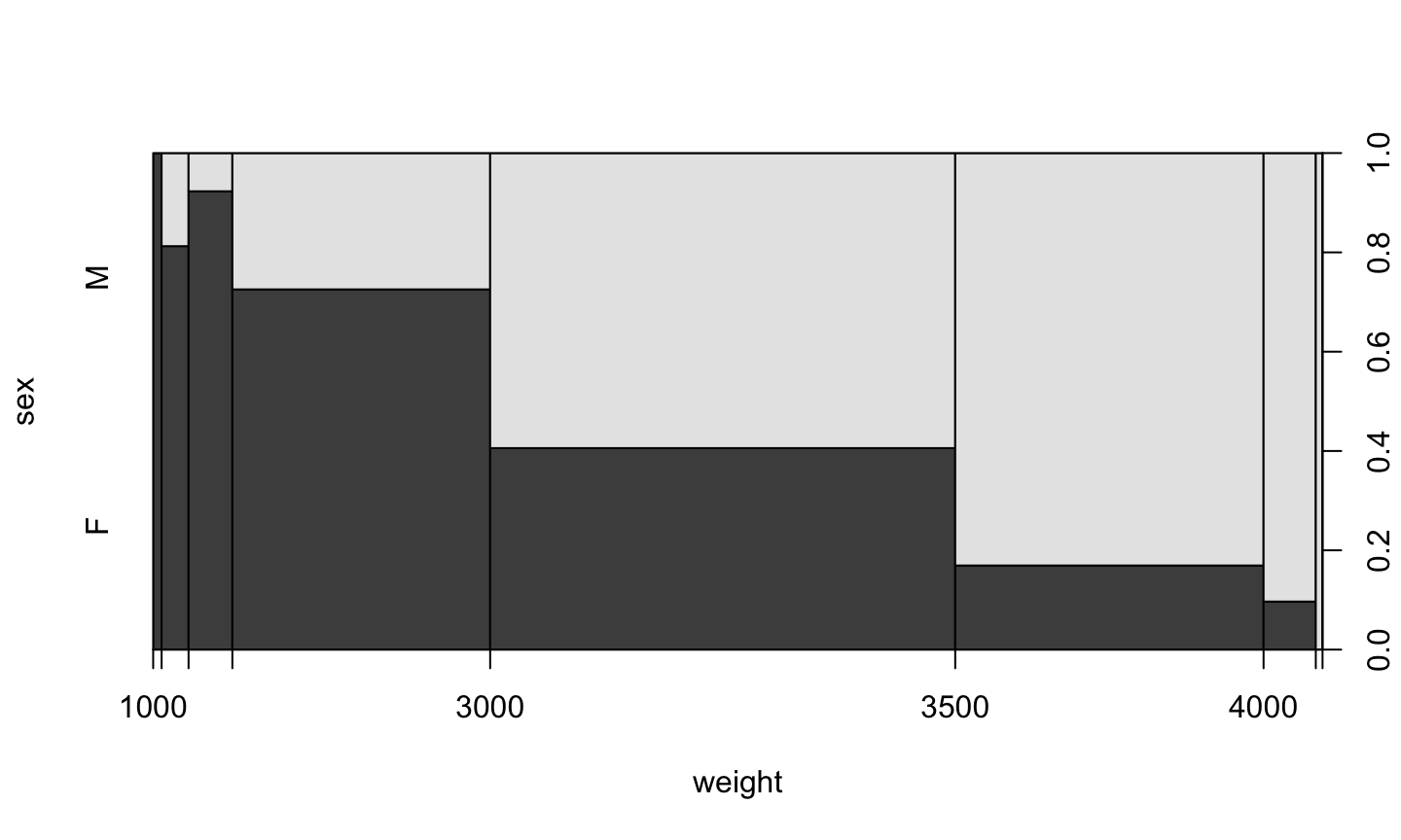
Factor v/s Numeric
plot(sex ~ weight, data=birth)
Saving graphics
Graphical Devices
By default all plot() commands work on a RStudio window
We can open a new device and redirect plot() output
Try this and check the Files window
pdf()
plot(sex ~ weight, data=birth)
dev.off()
Don’t forget to close the device!!
PDF, PNG, OMG!
There are many outpit devices
The most used are pdf() and png()
Try this and check the Files window
png()
plot(sex ~ weight, data=birth)
dev.off()
Don’t forget to close the device!!
What is the difference?
- PNG is a bitmap format: a bidimensional array of pixels
- other examples are JPG, TIFF, GIF
- PDF is a vectorial format: a mathematical description
- other example is SVG
The difference is seen when you zoom in
- PDF is good to print in paper
- PNG is better for screen and presentations
Multiple plots
Try this:
pdf()
plot(sex ~ weight, data=birth)
plot(weight ~ sex, data=birth, boxwex=0.2, notch=TRUE, col="grey")
plot(sex ~ apgar5, data=birth)
dev.off()
and look at the files.
What do you see?
Multiple plots
Now try this:
pdf(onefile=FALSE)
plot(sex ~ weight, data=birth)
plot(weight ~ sex, data=birth, boxwex=0.2, notch=TRUE, col="grey")
plot(sex ~ apgar5, data=birth)
dev.off()
and look at the files.
What do you see?
PDF options
pdf(file = ifelse(onefile, "Rplots.pdf", "Rplot%03d.pdf"),
    width, height, onefile, family, title, fonts, version,
    paper, encoding, bg, fg, pointsize, pagecentre, colormodel,
    useDingbats, useKerning, fillOddEven, compress)
- paper:
- “a4”, “letter”, “legal”, “executive”, “special”, “default”. Defaults to “special”
- width, height:
- specified in inches. Used when paper is “special”
- file:
- filename of the output file. Will be overwritten
PNG options
png(filename = "Rplot%03d.png",
    width = 480, height = 480, units = "px", pointsize = 12,
     bg = "white",  res = NA, ..., type, antialias)
- width, height:
- figure size, in “units”
- units:
- Can be px (pixels, the default), in (inches), cm or mm.
- res:
- The nominal resolution, in pixels per inch (ppi). Default 72.
- pointsize:
- the default pointsize of plotted text
- bg:
- the initial background colour: can be “transparent”.
But ploting many times is boring…
Functions in R
Whenever we need to execute the same set of commands more than 2 times, it can be useful to define a function
The format is:
new.function <- function(options) {
    command
    command
    ....
    command
    return(value)
}
Example
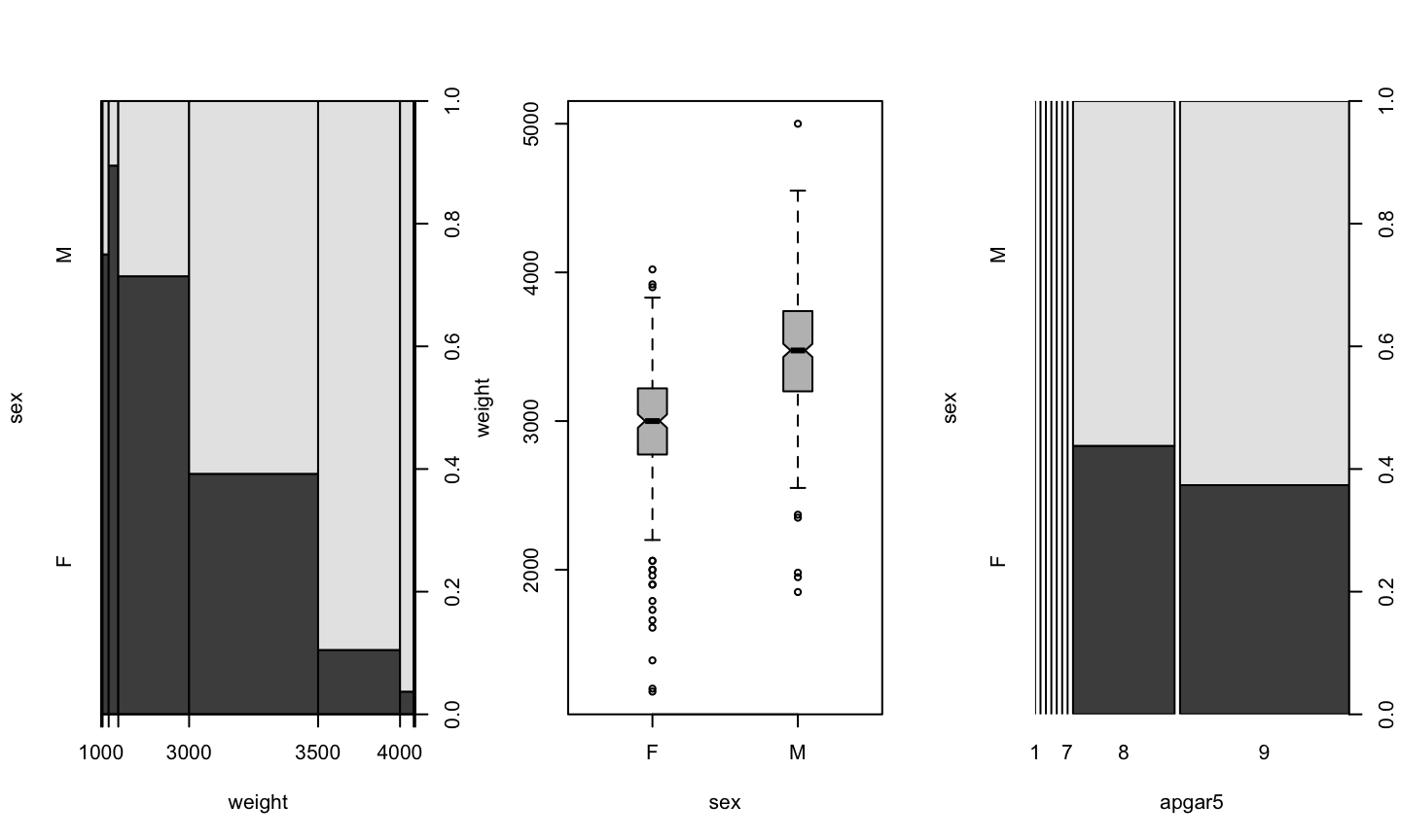
three.plots <- function() {
  plot(sex ~ weight, data=birth)
  plot(weight ~ sex, data=birth, boxwex=0.2, notch=TRUE, col="grey")
  plot(sex ~ apgar5, data=birth)
}
Using it
Try this, line by line:
three.plots()
pdf(file="three-plots.pdf", onefile=TRUE)
three.plots()
dev.off()
pdf(file="three-plots.pdf", onefile=TRUE)
par(mfrow=c(3,1))
three.plots()
dev.off()
Using it again
Try this now, line by line:
par(mfrow=c(3,1))
three.plots()
png()
three.plots()
dev.off()
png()
par(mfrow=c(3,1))
three.plots()
dev.off()
Passing values to the function
What if we want the same plots for different data?
For example, let’s define
healthy <- subset(birth, apgar5=="8" | apgar5=="9")
(how else can we build the data frame healthy?)
How can we draw the same plots for this data?
New data
summary(healthy)
       id            birth           apgar5    sex         weight
 Min.   : 4199   Min.   :1.000   9      :388   F:247   Min.   :1180
 1st Qu.: 6023   1st Qu.:1.000   8      :233   M:374   1st Qu.:2980
 Median : 7894   Median :1.000   1      :  0           Median :3250
 Mean   : 7836   Mean   :1.667   2      :  0           Mean   :3255
 3rd Qu.: 9601   3rd Qu.:2.000   3      :  0           3rd Qu.:3570
 Max.   :11475   Max.   :3.000   4      :  0           Max.   :5000
                                 (Other):  0
      head            age            parity          weeks
 Min.   :35.50   Min.   :22.00   Min.   :1.000   Min.   :29.00
 1st Qu.:48.00   1st Qu.:33.50   1st Qu.:1.000   1st Qu.:38.00
 Median :49.50   Median :34.50   Median :2.000   Median :39.00
 Mean   :49.37   Mean   :34.45   Mean   :2.599   Mean   :38.81
 3rd Qu.:51.00   3rd Qu.:35.50   3rd Qu.:4.000   3rd Qu.:40.00
 Max.   :55.00   Max.   :39.00   Max.   :9.000   Max.   :42.00
Redefining three.plots()
three.plots <- function(input) {
  plot(sex ~ weight, data=input)
  plot(weight ~ sex, data=input, boxwex=0.2, notch=TRUE, col="grey")
  plot(sex ~ apgar5, data=input)
}
New function
par(mfrow=c(1,3))
three.plots(healthy)
But now…
three.plots()
Error in eval(m$data, eframe): argument "input" is missing, with no default
It doesn’t work as before
Redefining three.plots() again
three.plots <- function(input=birth) {
  plot(sex ~ weight, data=input)
  plot(weight ~ sex, data=input, boxwex=0.2, notch=TRUE, col="grey")
  plot(sex ~ apgar5, data=input)
}
And now…
par(mfrow=c(1,3))
three.plots()
