Welcome back
to “Computing for Molecular Biology 1”
Plan for Today
- Graphics
- Adding elements
- Two variables
- Formulas
- Linear Regression
- R programs
Telling Stories
Data Visualization
plot(birth$weight)
 each individual has a position in the x axis
Ploting Factors
plot(birth$sex)

Histograms
par(mfrow = c(1,2))
plot(birth$head)
hist(birth$head, col="grey", nclass = 30)

Chosing the color
par(mfrow = c(1,2))
plot(birth$head)
plot(birth$head, col="red")

Chosing the size of the symbol
par(mfrow = c(1,2))
plot(birth$head, cex=2)
plot(birth$head, cex=0.5)

Chosing the symbol
par(mfrow = c(1,2))
plot(birth$head, pch=16)
plot(birth$head, pch=".")

Chosing the type of plot
par(mfrow = c(1,2))
plot(birth$head, type = "l")
plot(birth$head, type = "o")

Zooming
par(mfrow = c(1,2))
plot(birth$head, type = "l", xlim=c(1,100))
plot(birth$head, type = "o", xlim=c(1,100))

Full annotation
plot(birth$weight, main = "Weight at Birth", sub = "694 samples", ylab="weight [gr]")

Two plots in parallel
plot(birth$head)
points(birth$age, pch=2)
 The first one defines the scale
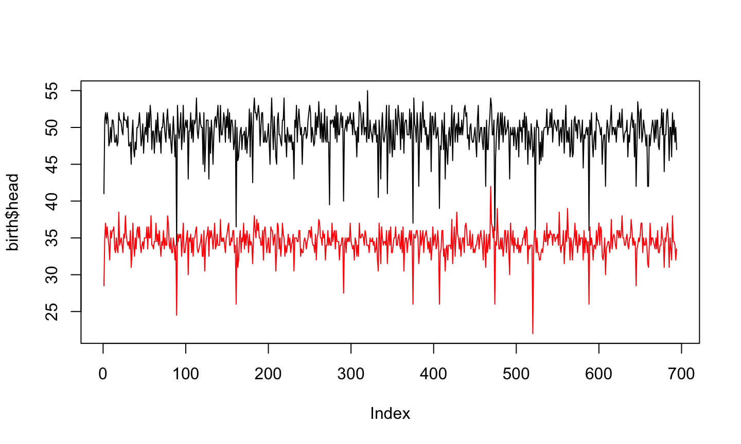
Two lines in parallel
plot(birth$head, type="l", ylim = c(22,55))
lines(birth$age, col="red")
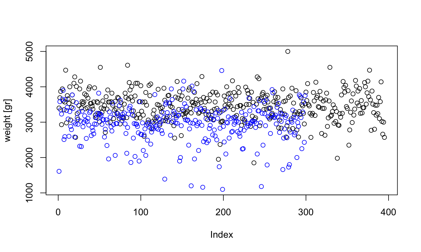
Boys and Girls
plot(birth$weight[birth$sex=="M"], ylim=range(birth$weight), ylab = "weight [gr]")
points(birth$weight[birth$sex=="F"], col="blue")
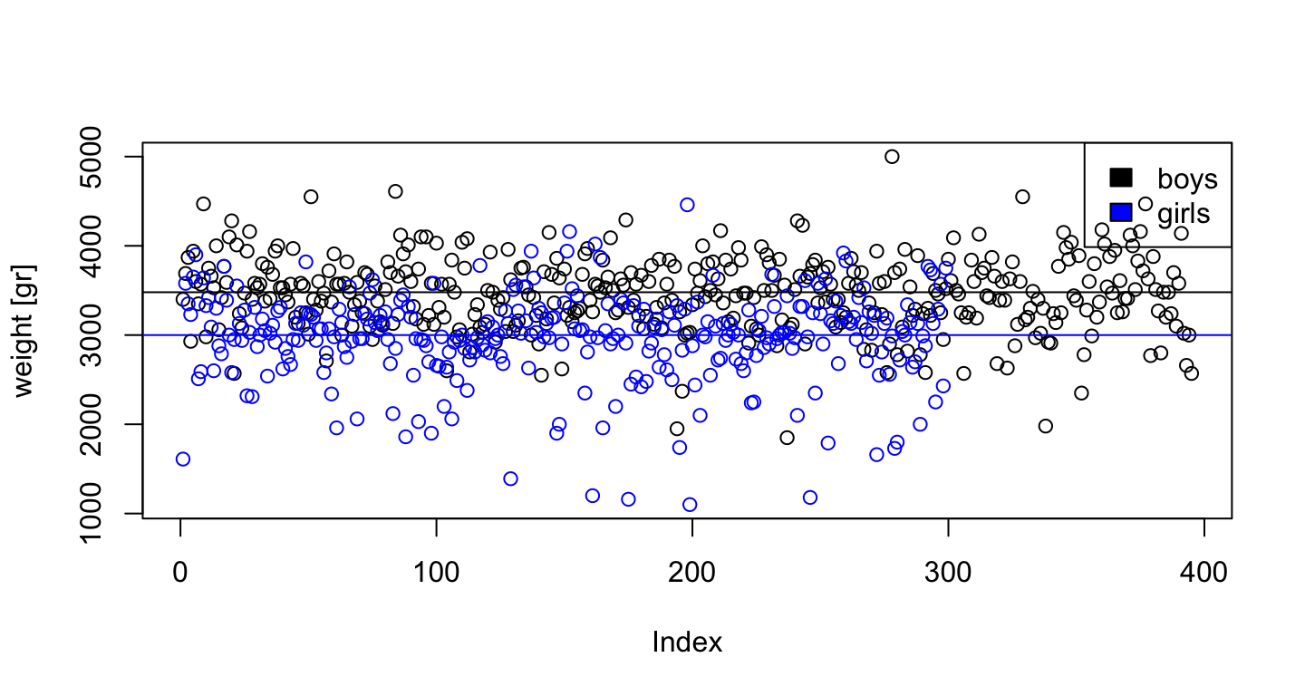
Using auxiliary variables
boys <- birth$weight[birth$sex=="M"]
girls <- birth$weight[birth$sex=="F"]
plot(boys, ylim=range(birth$weight), ylab = "weight [gr]")
points(girls, col="blue")
abline(h=median(boys))
abline(h=median(girls), col="blue")
legend("topright", c("boys","girls"), fill=c("black","blue"))
abline
This command adds a straigth line in a specific position
abline(h=1)adds a horizontal line in 1abline(v=2)adds a vertical line in 2abline(a=3, b=4)adds an \(a +b\cdot x\) line
Scatter plots
Comparing two variables
plot(birth$age, birth$apgar5)

Add jitter to see more
plot(jitter(birth$age), jitter(birth$apgar5))
 Less precise but more informative