Welcome back
to “Computing for Molecular Biology 1”
Telling Stories
Let’s recapitulate. We read data with
birth <- read.table("birth.txt", header=T)
which results in a data frame like this:
head(birth)
    id birth apgar5 sex weight head  age parity weeks
1 4347     1      8   F   1610 41.0 28.5      1    31
2 4346     1      9   F   3580 51.0 35.0      1    39
3 4300     1      9   F   3350 52.0 37.0      1    40
4 4345     1      9   F   3230 50.5 35.0      1    38
5 4349     1      8   F   3650 52.0 36.5      1    40
6 4315     2      8   F   3900 51.0 35.0      1    38
In summary
summary(birth)
       id            birth           apgar5      sex         weight
 Min.   : 4199   Min.   :1.000   Min.   :1.000   F:299   Min.   :1100
 1st Qu.: 6112   1st Qu.:1.000   1st Qu.:8.000   M:395   1st Qu.:2972
 Median : 7920   Median :1.000   Median :9.000           Median :3250
 Mean   : 7877   Mean   :1.677   Mean   :8.281           Mean   :3244
 3rd Qu.: 9606   3rd Qu.:2.000   3rd Qu.:9.000           3rd Qu.:3580
 Max.   :11475   Max.   :3.000   Max.   :9.000           Max.   :5000
      head           age            parity          weeks
 Min.   :34.0   Min.   :22.00   Min.   :1.000   Min.   :26.00
 1st Qu.:48.0   1st Qu.:33.50   1st Qu.:1.000   1st Qu.:38.00
 Median :50.0   Median :34.50   Median :2.000   Median :39.00
 Mean   :49.3   Mean   :34.42   Mean   :2.611   Mean   :38.75
 3rd Qu.:51.0   3rd Qu.:35.50   3rd Qu.:4.000   3rd Qu.:40.00
 Max.   :55.0   Max.   :42.00   Max.   :9.000   Max.   :42.00
What are these values?
Extrema
The easiest to understand are minimum and maximum
min(birth$weight)
[1] 1100
max(birth$weight)
[1] 5000
Which sometimes can be useful together
range(birth$weight)
[1] 1100 5000
Median
If m is the median of a vector v, then
- half of the values in
vare smaller thanm - half of the values in
vare bigger thanm
median(birth$weight)
[1] 3250
The median is the value \(m\) minimizes the absolute error \(\sum_{i=1}^n \vert v_i-m\vert\).
What if the number of elements is even?
Quartiles
Quart means one fourth in latin.
If we split the set of values in four subsets of the same size
Which are the limits of these sets?
\(Q_0\): Zero elements are smaller than this one
\(Q_1\): One quarter of the elements are smaller
\(Q_2\): Two quarters (half) of the elements are smaller
\(Q_3\): Three quarters of the elements are smaller
\(Q_4\): Four quarters (all) of the elements are smaller
It is easy to see that \(Q_0\) is the minimum, \(Q_2\) is the median, and \(Q_4\) is the maximum
Quartiles and Quantiles
Generalizing, we can ask, for each percentage p, which is the value on the vector v which is greather than p% of the rest of the values.
The function in R for that is called quantile()
By default it gives us the quartiles
quantile(birth$weight)
    0%    25%    50%    75%   100%
1100.0 2972.5 3250.0 3580.0 5000.0
quantile(birth$weight, seq(0, 1, by=0.1))
  0%  10%  20%  30%  40%  50%  60%  70%  80%  90% 100%
1100 2630 2906 3020 3140 3250 3388 3530 3660 3850 5000
Arithmetic Mean
The mean value of the vector v is \[\mathrm{mean}(v) = \frac{1}{n}\sum_{i=1}^n v_i\] where \(n\) is the length of v. Sometimes it is written as \(\bar{v}\)
mean(birth$weight)
[1] 3243.905
This value is usually called average, but the correct name is mean
This value minimizes the quadratic error \(\sum_{i=1}^n (v_i-\bar{v})^2\)
Mean of quadratic error
if \(n\) is the length of \(v\) and \(\bar{v}\) is its mean, then the mean of the quadratic error is \[\frac{1}{n}\sum_{i=1}^n (v_i-\bar{v})^2\] This number is called variance of the sample
This is a number in squared units, so it is hard to compare with the mean value
Variance and Standard Deviation
mean(birth$weight)
[1] 3243.905
var(birth$weight)
[1] 273438
To understand easily the variability of the data, we take the square root of the variance
The standar deviation of the sample is the square root of the variance \[\sqrt{\frac{1}{n}\sum_{i=1}^n (v_i-\bar{v})^2}\]
Variance and Standard Deviation
In many cases, including in R, people uses a slightly different formula \[\mathrm{sd}(v) = \sqrt{\frac{1}{n-1}\sum_{i=1}^n (v_i-\bar{v})^2}\] Explaining the reason is for a next course.
(It is because of the bias of the expected value of the expected value)
This value is called standard deviation of the population
Variance and Standard Deviation
The difference is small, especially when \(n\) is big
v <- birth$weight
sd(v)
[1] 522.913
sqrt(sum((v-mean(v))^2)/length(v))
[1] 522.5361
sqrt(sum((v-mean(v))^2)/(length(v)-1))
[1] 522.913
Data Visualization
“one image worths a thousand words”
Graphics
Sometimes the best way to tell the story of the data is with a graphic
plot(birth$weight)
 each individual has a position in the x axis
Another
plot(birth$head)

Ploting Factors
The previous graphics used numeric data. What about factors?
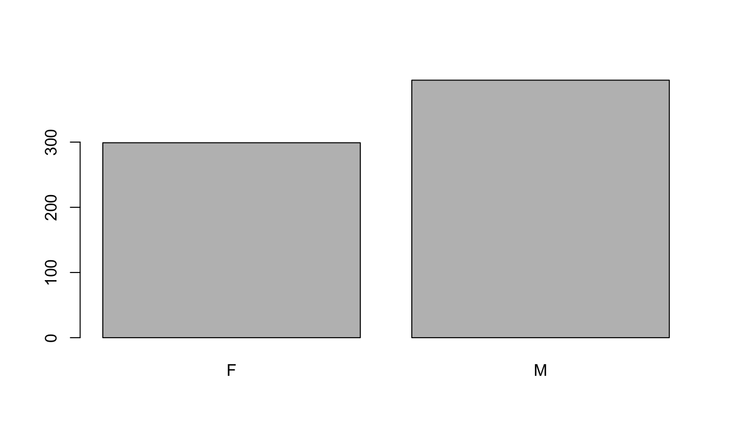
plot(birth$sex)
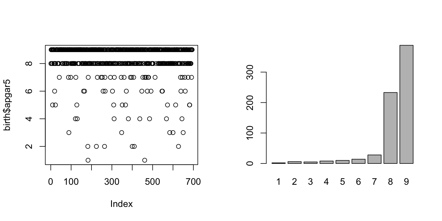
Apgar5: Number or factor?
par(mfrow = c(1,2))
plot(birth$apgar5)
plot(as.factor(birth$apgar5))
Histograms
par(mfrow = c(1,2))
plot(birth$head)
hist(birth$head)

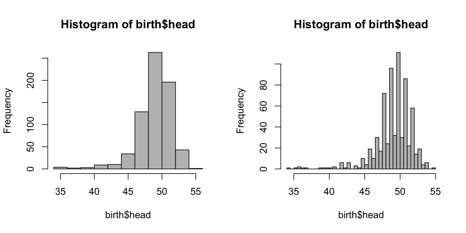
Histograms
Numeric data is grouped in N classes or bins
par(mfrow = c(1,2))
hist(birth$head, col="grey")
hist(birth$head, col="grey", nclass = 30)
Making it beautiful
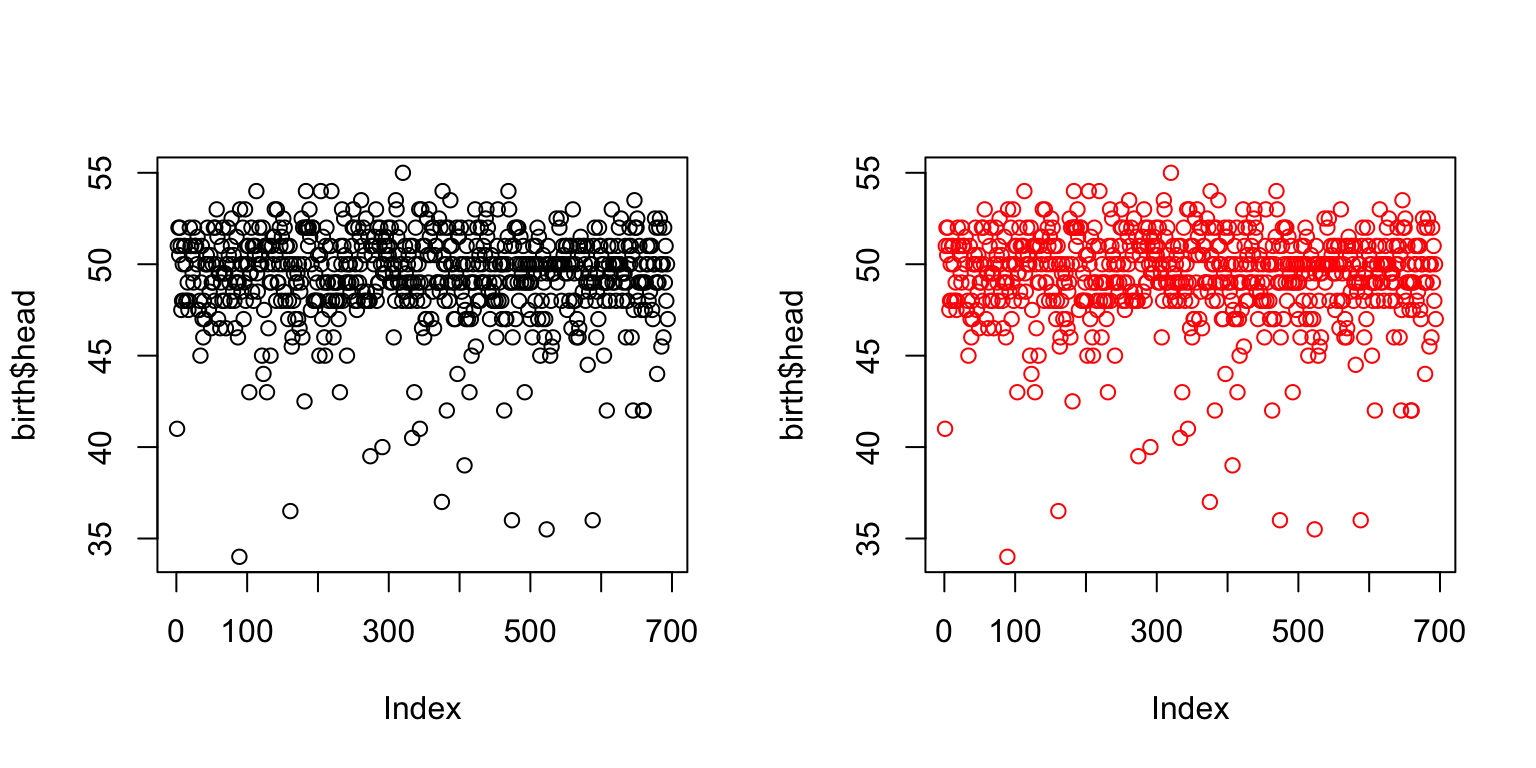
Chosing the color
par(mfrow = c(1,2))
plot(birth$head)
plot(birth$head, col="red")
Chosing the size of the symbol
par(mfrow = c(1,2))
plot(birth$head, cex=2)
plot(birth$head, cex=0.5)

Chosing the symbol
par(mfrow = c(1,2))
plot(birth$head, pch=16)
plot(birth$head, pch=".")

Chosing the type of plot
par(mfrow = c(1,2))
plot(birth$head, type = "l")
plot(birth$head, type = "o")

Zooming
par(mfrow = c(1,2))
plot(birth$head, type = "l", xlim=c(1,100))
plot(birth$head, type = "o", xlim=c(1,100))

More plot types
par(mfrow = c(1,2))
plot(birth$head, type = "b", xlim=c(1,100))
plot(birth$head, type = "n", xlim=c(1,100))

Full annotation
plot(birth$weight, main = "Weight at Birth", sub = "694 samples", ylab="weight [gr]")

Two or more variables
Two plots in parallel
plot(birth$head)
points(birth$age, pch=2)
 The first one defines the scale
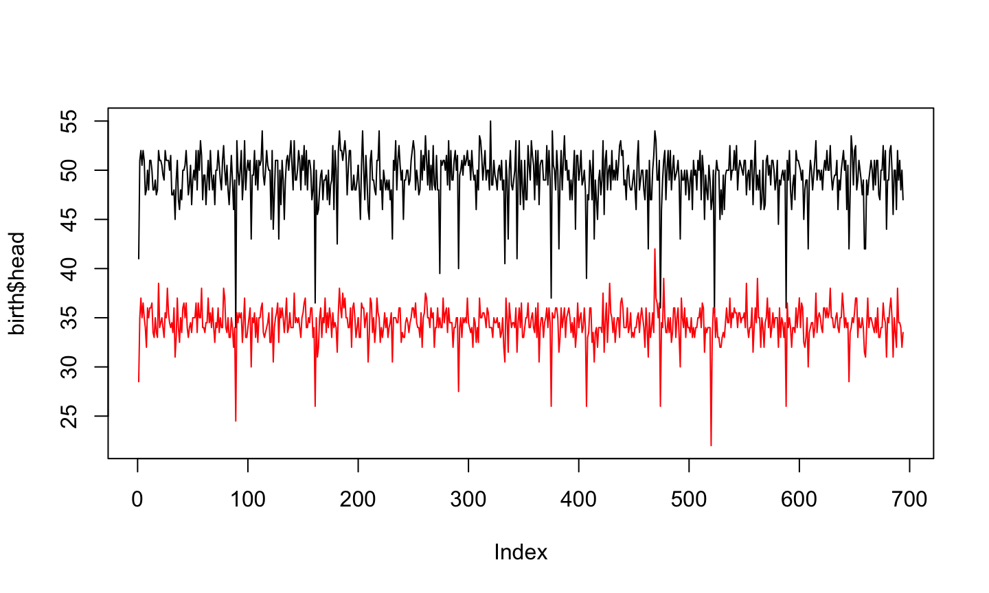
Two lines in parallel
plot(birth$head, type="l", ylim = c(22,55))
lines(birth$age, col="red")
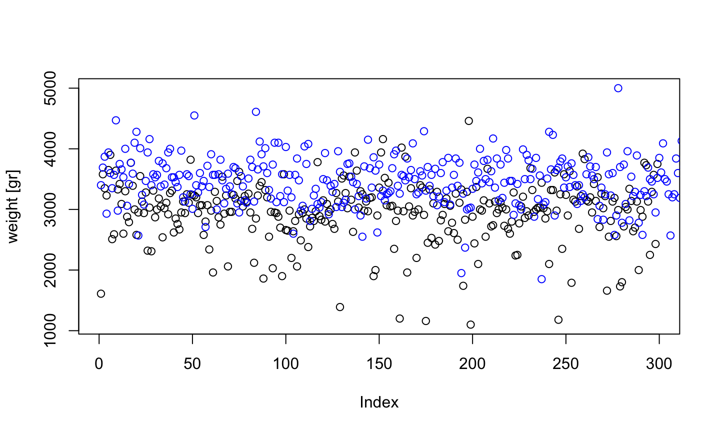
Boys and Girls
plot(birth$weight[birth$sex=="F"], ylim=range(birth$weight), ylab = "weight [gr]")
points(birth$weight[birth$sex=="M"], col="blue")