Please download the file quiz-5.R and write your results there. Send the your answers to my mailbox.
1 Genetic Algorithms
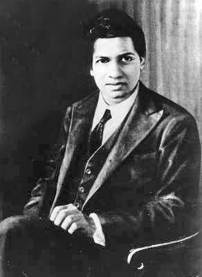
“Every positive integer was one of Ramanujan’s personal friends.” Srinivasa Ramanujan was an Indian mathematician born in 1887. Though he had almost no formal training in pure mathematics, he made substantial contributions including solutions to mathematical problems considered to be unsolvable. Ramanujan initially developed his own mathematical research in isolation. Seeking mathematicians who could better understand his work, in 1913 he began a postal partnership with the English mathematician G. H. Hardy at the University of Cambridge, England. Recognizing the extraordinary work sent to him as samples, Hardy arranged travel for Ramanujan to Cambridge. In his notes, Ramanujan had produced groundbreaking new theorems, including some that Hardy stated had “defeated (him and his colleagues) completely”, in addition to rediscovering recently proven but highly advanced results.
Throughout his life, Ramanujan was plagued by health problems. His health worsened in England. He was diagnosed with tuberculosis and a severe vitamin deficiency at the time, and was confined to a sanatorium. In 1919 he returned to Kumbakonam, Madras Presidency, and in 1920 he died at the age of 32.
One day that Ramanujan was sick at the hospital he was visited by his advisor. In Hardy’s words:
I had ridden in taxi cab number 1729 and remarked that the number seemed to me rather a dull one, and that I hoped it was not an unfavorable omen. “No”, he replied, “it is a very interesting number; it is the smallest number expressible as the sum of two cubes in two different ways.”
The two different ways are 1729 = 13 + 123 = 93 + 103. Can we do the same but for squares instead of cubes?
To be more specific, we are looking for a vector of integers \(v\) such that \[v[1]^2+v[2]^2=v[3]^2+v[4]^2\] Moreover, we want the two solutions to be different, thus \(v[1]<v[3]\) and \(v[1]<v[4].\) Obviously \(v[i]>0\) and \(v[i]\in \mathbb N\) for all \(i\).
We want to find a solution using genetic algorithms. Using the framework we saw in classes, please define
The file quiz-5.R has all the framework for genetic algorithms. You do not need wait until the programs find the solution. We only need the answers for these four questions.
2 Simulating Mendelian Genetics
G. H. Hardy, the advisor of S. Ramanujan The advisor of Ramanujan at Cambridge was Godfrey Harold Hardy, an English mathematician. His work was highly theoretical, and he was proud of doing “useless” mathematics1 However, his work in number theory is essential for ensuring the security of Internet commerce. His “useless” work is very practical today.. Nevertheless, he was the first mathematician who made a contribution to Biology and Genetics2 As you know, most of the mathematical tools in Biology were created by biologists.. Hardy co-discovered the Hardy–Weinberg principle, that states that allele and genotype frequencies in a population will remain constant from generation to generation in the absence of other evolutionary influences.
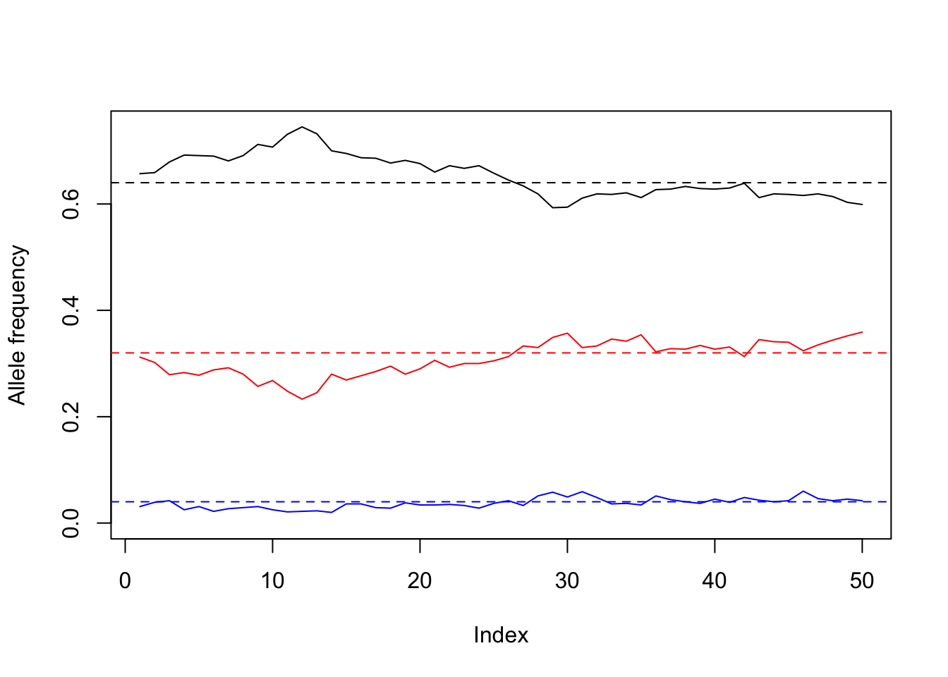
In the simplest case of a single locus with two alleles denoted \(A\) and \(a\) with frequencies \(f(A) = p\) and \(f(a) = q,\) respectively, the expected genotype frequencies under random mating are \(f(AA) = p^2\) for the \(AA\) homozygotes, \(f(aa) = q^2\) for the aa homozygotes, and \(f(Aa) = 2pq\) for the heterozygotes. In the absence of selection, mutation, genetic drift, or other forces, allele frequencies \(p\) and \(q\) are constant between generations, so equilibrium is reached.
This result was important because, at that time, people believed that a dominant allele would automatically tend to increase in frequency, confusion dominance and selection. That erroneous point of view was even used to justify racist policies, so Hardy’s result made the world a better place.
The Hardy–Weinberg principle describes the average behavior of the population. As we know, there is always some variability, and the real numbers may not match exactly the theoretical ones. In this exercise we want to test this.
We will simulate several generations of a population of N individuals, represented by the list pop. Each individual has only one locus, so we represent it by a vector with two allelic values. For example pop[[3]] can be c("A","a") while pop[[21]] can be c("a","a"). The probability of allele \(A\) is p. This will be done in a function called first_generation.
Each new generation replaces the complete population. There are no “survivors”. Every new individual has two randomly-chosen parents, and takes one allele from each parent randomly. This will be done in a function called new_generation.
We also need to count how many genotypes there are in the population. The function count_genotype takes the list pop and returns a numeric vector of size 3. The first element of the output vector is the number of times when pop[[i]] is c("A","A"). The third element of the output vector is the number of times when pop[[i]] is c("a","a"). As you may guess, the second element of the output vector counts the other genotypes.
The exercise has three parts:
Please write a function called first_generation with inputs N and p that returns a list with N vectors. Each vector has two elements. Each element is either "A" or "a", with probability p and 1-p, respectively.
Write a function called count_genotype that takes one input: the list pop. It must return a numeric vector of size 3. The elements of the output vector are: the number of times when pop[[i]] is c("A","A"), the number of times when pop[[i]] is either c("A","a") or c("a","A"), and the number of times when pop[[i]] is c("a","a").
Write a function called new generation that takes the list pop as an input and produces a new list of the same length. Every new individual has two randomly-chosen parents, and takes one allele from each parent randomly.
Most of the biographic text are based on the respective Wikipedia pages. The second exercise is based on a course by Dr. Mehmet Somel, Biology Department, METU.
 “Every positive integer was one of Ramanujan’s personal friends.” Srinivasa Ramanujan was an Indian mathematician born in 1887. Though he had almost no formal training in pure mathematics, he made substantial contributions including solutions to mathematical problems considered to be unsolvable. Ramanujan initially developed his own mathematical research in isolation. Seeking mathematicians who could better understand his work, in 1913 he began a postal partnership with the English mathematician G. H. Hardy at the University of Cambridge, England. Recognizing the extraordinary work sent to him as samples, Hardy arranged travel for Ramanujan to Cambridge. In his notes, Ramanujan had produced groundbreaking new theorems, including some that Hardy stated had “defeated (him and his colleagues) completely”, in addition to rediscovering recently proven but highly advanced results.
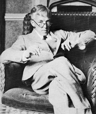 G. H. Hardy, the advisor of S. Ramanujan