Keywords
- Fragments
- Fragment size
- Libraries
- Adaptors, vectors
- Reads
- Read length
- Single end
- Paired end
- Mate pairs
- Base calling
- Phred Quality
- Trimming by quality
- Clipping adaptors/vectors/tags
- Contigs
- Depth
- Overlap Threshold
- Scaffolds
- Repeats
Note: My experience is mainly on the Sanger sequencing method and first generation assemblers. Moreover, I have worked mostly on Bacteria. Therefore this document is not complete. It is true, but does not include everything. We have to learn together about New Generation Sequencers and modern DNA assemblers.

A soldier splitting a target using shotgun
1 Sequencing DNA
Current technology for DNA sequencing cannot process a complete chromosome. Instead, we have to break the DNA into smaller fragments.
We can break the chromosome in several ways. The most common method is to sonicate them: using ultrasound the chromosome is broken at random places. This method is called shotgun, because the DNA is split in any position, like the bullets coming out of a shotgun.
In the typical protocol for Sanger sequencing, the fragments are separated by size using gel electrophoresis. Using a ladder as a guide, fragments of a given size are selected and inserted into cloning vectors (a particular kind of plasmid). For example one library can be made with 2kbp fragments, and another with 10kbp fragments. In this context library means a collection of fragments of approximately the same size. The cloning vector is inserted into a host cell, such as E.coli. When the cells duplicate, the plasmid also duplicates. Eventually this results in several million copies of the same fragment.
Homework: Find the sequence of any cloning vector and identify its parts.
Fragments are usually identified by a tuple (organism, plate, row, column) that corresponds to the physical location of the clone. Laboratories that follow good practices register this in a special database: a laboratory information system, also known as LIS.
2 Chromatograms in Sanger method
Sanger method reads DNA using capillary electrophoresis. Each clone is amplified using PCR. For that, the cloning plasmid has pre-defined primers that only amplify the inserted fragment. At this stage we have several million copies of the same fragment. They are separated into four parts, and each part is digested with different restriction enzymes that cut them in specific nucleotides. One group is split on an A nucleotide, the second is split on C, the third on G, and the last on T. Then each aliquot is marked with different fluorophores.
Finally all the aliquotes are mixed and run through capillary electrophoresis in front of a light detector. The device detects the intensity for each of the colors corresponding to each nucleotide. The result is a chromatogram, that literally means writing colors.
Chromatograms are stored in .abi, .ab1, or .scf files, and can be read with programs such as Codon Code or, more usually, phred.
This procedure can be repeated for the other side of the fragment. In most cases we get two chromatograms for each fragment
3 Base calling and preprocessing
The next step is to identify each nucleotide in the chromatogram. This process is called base calling. Several programs can do that, including:
phred- TraceTuner
- Tracy
seqretfrom the EMBOSS suite
This step produces two results for each chromatogram: the bases detected from the signals, and a quality value for each base. The quality is an assessment of the confidence of each letter. Higher values correspond to higher confidences. The figure shows the quality value for each predicted nucleotide on a Sanger read
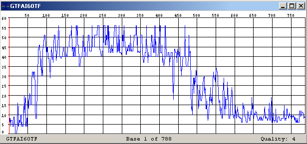
Figure: Plot of quality value for each base in the read GTFAI60TF
Homework: learn some of the quality values and their meaning.
3.1 Phred Quality
Essentially, they quality is the probability that the base calling is wrong. If you are an Audio addict, you can also see it as the signal-noise ratio measured in decibels. The first program to use this measure was Phred, so these are called Phred qualities.
In this model, the quality value is the integer part of -10*log(Probability(error)). That is, you take the probability of error, you calculate its logarithm (in base 10), you multiply the result by -10, and then you take the integer part. The following table shows some typical quality values:
| P(correct) | P(error) | log10(P(error)) | -10 times |
|---|---|---|---|
| 90.0% | 0.1 | -1 | 10 |
| 95.0% | 0.05 | -1.3 | 13 |
| 98.0% | 0.02 | -1.7 | 17 |
| 99.0% | 0.01 | -2 | 20 |
| 99.9% | 0.001 | -3 | 30 |
| 99.99% | 0.0001 | -4 | 40 |
| 99.999999% | 0.00000001 | -8 | 80 |
The sequence of bases and their quality values are then stored in a new file. Several file formats can be used. Today the most common one is FASTQ.
3.2 FASTQ format
The result of the base-calling step has to be stored in a file. There are several formats to store this information, including the original phred format. Today the most common way to store predicted bases and their qualities is FASTQ.
Files in FASTQ format are text files. Thus, they are easy to read and understand. One file can contain several reads. Each read is represented by a record in the file. This format is based on the FASTA format, but with some important differences. Let’s look at the next example:
@SEQ_ID
GATTTGGGGTTCAAAGCAGTATCGATCAAATAGTAAATCCATTTGTTCAACTCACAGTTT
+
!''*((((***+))%%%++)(%%%%).1***-+*''))**55CCF>>>>>>CCCCCCC65
All FASTQ records follow the same pattern, which is this:
@ ID [description]
SEQUENCE
+
quality
As in FASTA files, each record stats with a marker character. Instead of starting with >, FASTQ records start with @. Like in FASTA, this starter character is immediately followed by the read identification, and optionally a description. Then, like in FASTA, the second line has the nucleotide sequence. In theory, the nucleotide sequence can wrap and use more than one line, but in most cases all the sequence is written in a single line.
The first important difference between FASTA and FASTQ is that the last ones includes qualities. For that, the third line of a FASTQ record is a single + character and the fourth line has the qualities as a text of the same length as the sequence. Each character represents a quality, according to a simple rule: their position in the following lines
!"#$%&'()*+,-./0123456789:;<=>?@ABCDEFGHIJKLMNOPQRSTUVWXYZ[\]^_`abcdefghijklmnopqrstuvwxyz{|}~Thus, a quality 0 will be represented by !, while a quality of 25 will be represented by :.
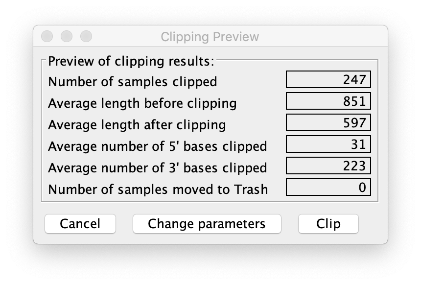
Report of clipping reads on CodonCode Aligner. Few bases clipped at 5’ end, many more at the 3’ end
3.3 Clipping and Trimming
The last step in this quality control stage is to discard the wrong nucleotides. There are two reasons for doing this.
The first one is to discard low quality letters at the beginning and the end of the read. As we saw in the Figure 3, the first few and the last several bases have lower quality, so they are more noise than signal. It is recommended to clip the reads and remove low quality nucleotides from the 5’ and the 3’ extreme. A reasonable quality value to use as clipping threshold is 10.
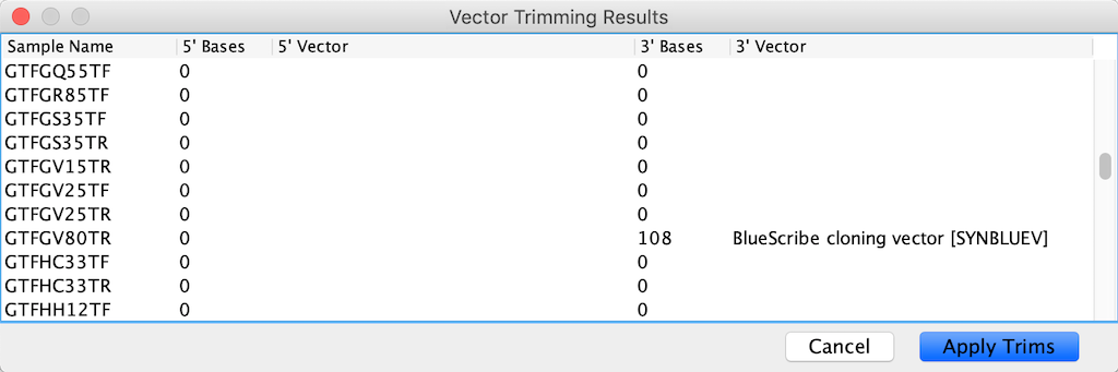
Report of vector Trimming results on CodonCode Aligner. Only a few reads had remains of the cloning vector.
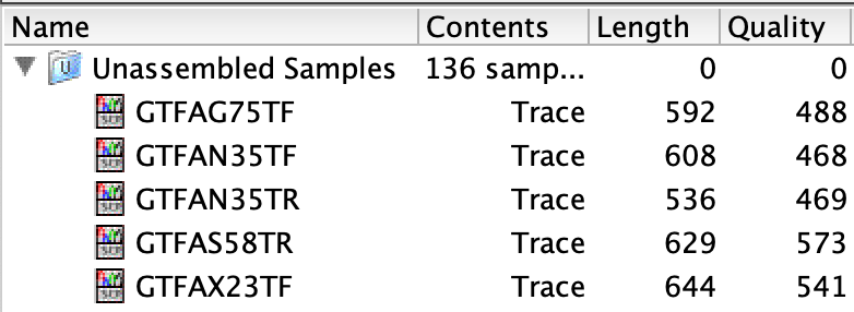
Read length is reduced after clipping and trimming. The remaining bases have good quality and are biologically relevant.
The second step is to see if part of the cloning vector or adaptor has been accidentally sequenced. As we know, different sequencing method use different molecular techniques. Most of them use PCR and require specific primer binding sites. These sites are called adaptors. In the Sanger method they are part of the cloning vector. Clearly, they are not part of the genome we want to sequence. Indeed, they are a technical artifact and they should not be used in the next step. Otherwise we risk to confuse the assembler and produce chimeric sequences.
To do vector trimming we need to compare every read to the sequences of known adaptors. We use a small database with the sequences of standard vectors and adaptors.
4 De novo assembly
Once we got good quality reads, the next step is to combine them into longer sequences. This is done with programs that compare all reads and check if the last nucleotides of one read match the first nucleotides of another read. When this happens, we say that there is an overlap.
We must say that there is a new generation of assemblers that does not work with reads, but with fragments of reads. This strategy is known as De Bruijn graphs and we will not study it in this course.
4.1 Overlap Threshold
To detect that two reads are part of the same genome region, assemblers check if the last nucleotides of one read match the first nucleotides of another read. When this happens, we say that there is an overlap.
It is easy to see that this can induce errors, unless we discard very short overlaps. If the overlap size is small, it is easy to find the same short sequence in two reads just by (bad) chance. If that happens, the genome assembler may erroneously put together reads that belong to different regions of the genome, that are not close in reality. When that happens, we say that there is a chimeric assembly.
Without any additional biological knowledge, we can estimate the probability that two reads overlap on T letters as \[P(\text{overlap length T})=4^{-T}.\] When we have \(N\) reads, we have to compare every one to each other. That is, we have to check \(N(N-1)\approx N^2\) pairs. Combining this two formulas, we can find the expected number of chimeric assemblies for an overlap threshold \(T\) as \[E(\text{number of chimeric assemblies})\approx N^2\cdot 4^{-T}\] For example, if there are \(10^5\) reads, the expected number of chimeras, depending on threshold value \(T\) is
| T | Chimeras |
|---|---|
| 5 | 9765625 |
| 10 | 9537 |
| 15 | 9.313 |
| 20 | 0.009 |
4.2 Contigs
A contig is a set of reads that overlap. The name comes from the fact that they represent a contiguous part of a chromosome. The assembly program uses these reads to determine their relative position, called layout. Combining reads and layout the program produces a consensus sequence: the bases of each position of the contig, and their quality.
4.3 Scaffolds

This is the everyday meaning of scaffolds.
In most cases each DNA fragment is sequenced twice, one time for each extreme. We get two reads for each fragment, oriented forward and reverse. Since the reads belong to the same fragment, this gives us some extra information: these two reads are physically close.
When the forward read is located in a different contig than the reverse read, this extra information allows us to know the relative position of each contig. We say that the two contigs are linked by one or more fragments. Following this idea we can connect several contigs into a bigger structure called scaffold.
Finding scaffolds is good for several reasons. First, it contain contigs that belong to the same chromosome, so we get an idea of the chromosome structure. We can use extra information, such as genetic markers or gene linkage to validate or extend the scaffold. The scaffold structure can be validated by doing PCR between contigs that are in theory side by side.
Second, a scaffold is a kind of “big contig with gaps”. The regions between contigs are called gaps. We do not know the value of the bases there, but we know its length, more or less. This allows us to design PCR primers on each side of the gap, inside the contigs, and then amplify and sequence the gap. Normally “gap closing” is the last stage of a sequencing project. Nevertheless many projects, including the human genome, are declared complete even when some gaps still exist in the scaffold.
Some parts of the chromosomes are harder to sequence, such as telomers and centromers. In those cases researchers are happy with an assembly that has one scaffold for each chromosome, and over 99% of the bases are known. The unknown bases are represented by N, as you can see in this example:
>NC_005108.4 Rattus norvegicus strain mixed chromosome 9, Rnor_6.0
TCCACTAACTCTGTTACAAGGAGGGGAGAGAACAGTAAATTGCTTCTGTTACTGAGATCATCTGGAAGTT
GAACTATTTCCTACAGGTGTAACTTTGTTTAGCCCACTGGGAAAGAGATGCTAGATCAGCTCTTGGAAAC
CTTAGCCATAGAGAGAAACCTCAGTGTGAAACTCCAGCTGATGCTTAAACTTCCTCAGTTTCTTGAAAAT
GGTGTGAGCACAGGATCTCCTGATGTTATCTCTTTCCTACCAGTCCTTTACTTGGAGGAATACTCTGCTC
AGCCTGGGTATTTTATGAGTAAACTGACTGGCTATCCCAATGGAGATTCATCAGTAGTTTTTGCTAGATG
TTTGTGAGTCCTCCCCTTGTAATATTATCTTTCTACTGTGATTTGTTCCTTGACCTGGAAGCCGTGCCCA
GGGACACACTATGCTCTGCCTGGGAATCTCAGTGCTGGGAACACAAAGTGTCAGATTCAAGAGGGCTTGT
CCAGGCAATTTCTGCTTGAGGACCTGATTTGTNNNNNNNNNNNNNNNNNNNNNNNNNNNNNNNNNNNNNN
NNNNNNNNNNNNAAGAAATACAGCAGACTTCTCACCAGATTCTATGAATGCCAGAAGGTCCGGGGCAGAT
5 References
- Chou, H.-H., and M. H. Holmes. “DNA Sequence Quality Trimming and Vector Removal.” Bioinformatics 17, no. 12 (2001): 1093–1104. doi:10.1093/bioinformatics/17.12.1093.
- Sims, David, Ian Sudbery, Nicholas E. Ilott, Andreas Heger, and Chris P. Ponting. “Sequencing Depth and Coverage: Key Considerations in Genomic Analyses.” Nature Reviews Genetics 15, no. 2 (2014): 121–32. doi:10.1038/nrg3642.
- Nagarajan, Niranjan, and Mihai Pop. “Sequence Assembly Demystified.” Nature Reviews. Genetics 14, no. 3 (2013): 157–67. doi:10.1038/nrg3367.
- Lander, E S, and M S Waterman. “Genomic Mapping by Fingerprinting Random Clones: A Mathematical Analysis.” Genomics 2, no. 3 (April 1, 1988): 231–39.