Final Exam with Answers
Computing in Molecular Biology 2 — Molecular Biology and Genetics Deptartment
2nd of June, 2017
Please download the answer file and edit it on Rstudio. You should be able to Knit HTML and get the same results as the document you have in paper. Please do Knit often and verify that your document has no errors. If your document does not Knit, you will not have full grade.
When you finish, send the answers.Rmd file to my mailbox. Be sure to use the correct email address and send only one file. If you send the wrong file your grade will be 0. Please ask me if I received the file before closing your computer.
You can use your personal handwritten notes and the help window of RStudio. All questions are independent and can be answered in any order. Some question can be answered in more than one way. Only one correct answer is required.
IMPORTANT: Write your student number in the correct place at the beginning of the answer file.
All answers are strictly personal. Any unethical behavior will be penalized.
In this Exam we will analyze the genome of Candidatus Carsonella ruddii PV, which is the smallest one in bacteria, published by Nakabachi et al. “The 160-kilobase genome of the bacterial endosymbiont Carsonella.” Science (2006) 314:267.
You must download the genome of C. rudii from the web, either form NCBI or from the website of the course. You will need the files AP009180.fna and AP009180.gff. Store both files on the same folder where you stored the answer.Rmd file.
You can load the genome with the following command (do not change it):
1 (15%) GC content
Please write the code to determine the GC percentage of C.ruddii. Your code should produce this result
This was easy because we had seen it on classes. Nevertheless many people gave long answers with functions and loops that are not necessary. If you understand then the answer is short and easy.
Here we only need code, not any function. If you write a function then you have to use it and show the result.
[1] 16.564372 Four-letter words
We know that the frequency of each codon (that is, words of size 3) is an important characteristic of each organism. We want to explore the same idea for words of size 4.
2.1 (15%) Count and Draw
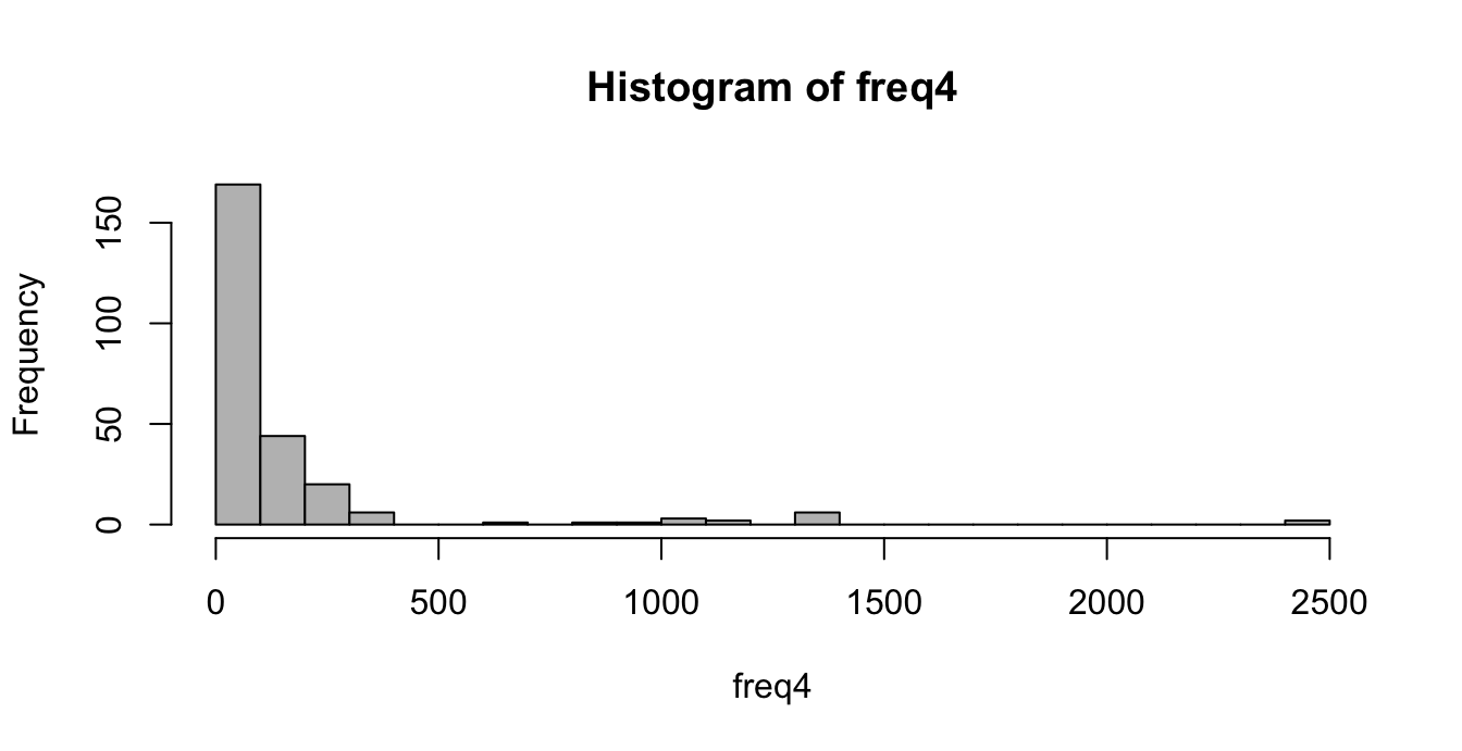
Please write the code to count how many times each word of size 4 appears in the full genome of C. ruddii. The function splitseq() may be useful. Store that result in the variable freq4.
Here most people understood that we need to use the function
splitseq()with the optionword=4. But many people forgot to count them using thetable()function, and assign them tofreq4. Both steps are necessary.
You should get this histogram:
2.2 (10%) Most frequent words
In the previous histogram we can see that only a few 4-words have high frequency. Write the code to show the name and frequency of the 4-words with frequency greater than 500.
This is just a simple application of what we studied on the last semester.
It is essential to learn the subject, not only to memorize it for the exam.
aaaa aaat aata aatt ataa atat atta attt taaa taat tata tatt ttaa ttat ttta tttt
2445 1366 1111 1376 1032  812 1061 1373 1340  952  647 1158 1321 1003 1303 2425
2.3 (bonus) What do these words have in common?
The most frequent words do follow a pattern. What is it? What is the biological reason for it?
- All the most frequent words have only A and T. There are no G or C. That is because the %GC content is very low
- The reverse-complement of each frequent word is also a frequent word.
- Moreover, the frequency of each word is very similar to the frequency of its complement
- This is because nature has no preference for any strand. Anything that happens in one strand do also happen in the other.
Notice that words of length 4 are not related to translation of genes into proteins. Thus, any mention of “codon” is nonsense.
3 Replication Origin
3.1 (15%) GC skew
Write a function called get_gc_skew that get a vector of char representing dna and returns the difference between the number of “g” and the number of “c” nucleotides in dna.
We had seen this in class and in a homework. It is essential to use
tableand to evaluatefreq["g"]-freq["c"].This was the only question that asked for a function. In all other cases you only need to write the code, without defining a new function.
If everything is right your function should give this result:
g
3
Some people returned
freq["g"]-freq["c"]divided bylength(dna)or bysum(freq), but that was not necessary. In the example you see that the result is an integer number and you can even count “by hand”.In any case, if you divided or not did, it did not changed your grade.
3.2 (15%) Cumulate GC skew
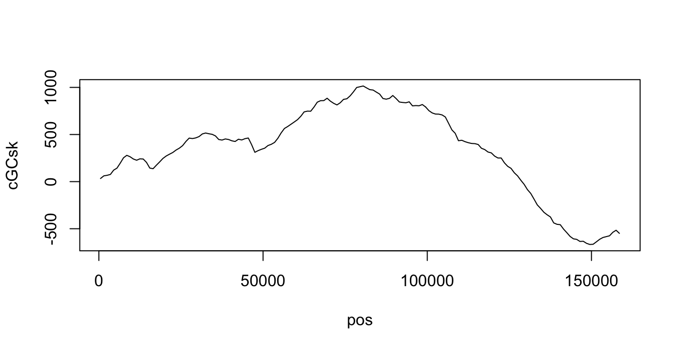
Calculate the cumulative GC skew for the genome of C.ruddii in steps of 1000 nucleotides. That is, take the genome in pieces of size 1000, calculate the GC skew for each piece (using the function get_gc_skew()) and store it on GCsk. Then calculate the cumulative sum of the GC skew and store it on the vector cGCsk. Remember that the cumulative sum cGCsk at position i is the sum of the cumulative sum at position i-1 plus the GC skew GCsk at position i.
For your convenience, the first lines of the code are given here. You have to complete the code. Do not forget to store the position of each piece in the vector pos.
The answer to this question was the longest. But, as many people realized, we saw it in class so it was not really hard. The key parts are:
- using a
forloop- update
cGCsk[i]based oncGCsk[i-1]- update
startandendon each stepThere is an alternative solution using
cumsum()function
step_size <- 1000
N <- as.integer(length(genome)/step_size)
pos <- rep(0, N)
GCsk <- rep(0, N)
cGCsk <- rep(0, N)
start <- 1
end <- step_size
pos[1] <- start + step_size/2 -1
cGCsk[1] <- get_gc_skew(genome[start:end])
for(i in 2:N) {
  start <- start + step_size
  end <- end + step_size
  pos[i] <- start + step_size/2 -1
  cGCsk[i] <- cGCsk[i-1] + get_gc_skew(genome[start:end])
}
The result should be like this
3.3 (15%) Where is the Origin of Replication?
During mitosis, the DNA of C.rudii is replicated starting from the origin of replication. It is located either at the minimum or maximum of the cGCsk curve. Please write the code to determine the possible locations of the origin of replication in the chromosome of C.rudii.
Here most people got the correct intuition: you have to look for the extreme values of
cGCsk. But many people got confused betweenmax(cGCsk),which.max(cGCsk)andpos[which.max(cGCsk)].
- When you use
max(cGCsk)you get the biggest value ofcGCsk.- When you use
which.max(cGCsk)you get the index of the biggest value.- When you use
pos[which.max(cGCsk)]you get the position of the biggest value, and that was the correct answer.Again, this shows that most people did not practice enough. You need to do all exercises and homework, and then many more.
[1] 149500 80500You can answer this question even if you did not answered the previous one.
4 Genes
Now we want to take a look at the genes of C.rudii. For that, we need to load the annotation using the following code:
gff <- read.table("AP009180.gff", comment.char = "#",
          header=FALSE, sep="\t", quote = "", as.is=TRUE,
          col.names=c("seqname", "source", "feature", "start", "end",
           "score", "strand", "frame", "attribute"))
Here we load a GFF file, not a FNA file. This is not the same as we did in class. The exam evaluates how you think, not how you remember.
4.1 (15%) Length of genes
Find the subset of gff where the column feature is equal to "gene" and store it on a new data frame called genes. Then calculate the length of each gene and store them on a vector named len.
The first step is to create the
genesdata frame. Most people got it right, since we saw it in class.The second step is very easy if you understand the GFF format. We saw it in classes, and you can read more on the web.
Notice that there is a
+1at the end to get the correct length (but if you forgot it does not affect your grade).An alternative solution can also be done using a
forloop and adapting the example we saw on classes. You first get the gene from the genome (which you had from the previous question) and then you measure its length. Both approaches are valid, although the first is easiest and less error-prone.
N <- nrow(genes)
len <- rep(NA, N)
for(i in 1:N) {
    gene <- genome[ genes$start[i]:genes$end[i] ]
        len[i] <- length(gene)
}
You should get this summary:
   Min. 1st Qu.  Median    Mean 3rd Qu.    Max.
   71.0   264.0   540.0   736.5  1047.0  3879.0
4.2 (15%) Longest gene
Write the code to show the details of the longest gene. The result should be this
       seqname source feature  start    end score strand frame
406 AP009180.1   DDBJ    gene 137484 141362     .      -     .
                                                                           attribute
406 ID=gene188;Name=CRP_161;gbkey=Gene;gene_biotype=protein_coding;locus_tag=CRP_161
Here most people understood that we need to use some kind of maximum. But again there is confusion about the exact way to use it. For example:
max(len)gives us the length of the longest gene.which.max(len)gives us the index of the longest gene.genes[which.max(len),]gives us the details of the longest gene.Notice that
genesis a data frame, so we can use a 2-dimension index. In this case we specify the row, then we write a comma and then we leave empty the column-index. That gives us all columns for one row.Again, this is something you should know from the last semester. You probably should re-do all the homework from last semester and this semester.