Some R code is not essential to the discussion. They are still interesting, so they are included as margin notes.
In the previous article we discussed the application of linear models to predict what will happen in conditions that we have not seen before. The assumption is that there is an underlying mechanism behind the observed values, plus some random noise. Moreover, we assume that the underlying mechanism is linear. This is not always the case, but it is a valid assumption in many cases. And it is always a good starting point.
We use linear regression to find the parameters that define the behavior of such mechanism. We can then predict what will happen, as we did in the previous article. In other cases we are interested in the parameters of the linear model, because they have an interpretation.
In this article we are going to analyze two experiments intended to measure physical values represented by parameters of linear models.
Speed of sound
echo_delay <- read.delim("echo_delay.txt")We will analyze the results of the sound speed experiment,
contained in the file echo_delay.txt.
There are 527 samples and 4 variables. The following table shows the
first and last four rows
kable(echo_delay[c(1:4, nrow(echo_delay)-3:0),])| id | elapsed | delay | distance | |
|---|---|---|---|---|
| 1 | 3 | 1 | 105 | 12 |
| 2 | 4 | 2 | 104 | 12 |
| 3 | 5 | 2 | 106 | 12 |
| 4 | 6 | 3 | 106 | 12 |
| 524 | 640 | 378 | 1056 | 180 |
| 525 | 641 | 379 | 1055 | 180 |
| 526 | 642 | 380 | 1055 | 180 |
| 527 | 643 | 380 | 1055 | 180 |
The column id is the sample serial number. Some cases have
been omitted, as described in the experiment protocol document. The
column elapsed represent how many seconds passed since the
start of the experiment until the sample was taken. It is used for data
pre-processing and quality control, but it is not needed for the current
analysis. In this case, the most important variables are delay
and distance. The variable delaydelay: units 10-6s,
resolution ±0.5
is the number of microseconds that passed between sending
the ultrasonic signal and receiving the echo. The resolution is one
microsecond. There is some variability that shall be treated
statistically.
The variable distancedistance: units 10-3m,
resolution ±0.5
is the distance between the sensor border and the wall
where the echo bounces. The total traveled distance is twice this value.
It is measured in millimeters, with a margin of error of 1mm. There may
be an unknown offset between the real position of the sensor
and the place used as reference for distance.
Their relationship is, by definition, given by \[speed\cdot delay
=2\cdot(\mathit{distance}+\mathit{offset})\] Remember that the
sound travels distance twice. We can rewrite this formulaIn principle we can also use the model \[{distance}=2\cdot speed\cdot
delay+\mathit{offset}\] but it is harder to analyze, since
delay is not the variable that we control. Instead we control
distance.
in a more convenient way as \[\mathit{delay}
=\frac{2}{\mathit{speed}}\cdot\mathit{distance}+\frac{2\cdot
\mathit{offset}}{speed}\] This formula has the shape of a linear
model \[\mathit{delay}
=\beta_1\cdot\mathit{distance}+\beta_0\]
Fitting the model will give us two parameters: an intercept \(\beta_0\) that will correspond to the 2 offset/speed, and a factor for distance that will correspond to 2/speed.
For some distances we have several samples, while in others we have only a few. We have to take them in consideration when we fit the linear model, since the cases with more samples will have more weight than the cases with fewer samples.
plot(delay~id, data=echo_delay,
    main="Delay [ms] for each sample")
We have to count the number of samples in each case
num_samples <- table(echo_delay$distance)
num_samples
12 20 30 40 50 60 70 80 90 100 110 120 130 140 150 160 170 180
67 25 25 23 24 42 19 11 27 31 26 20 43 27 29 25 25 38 Now we can fit a linear model to this data, including weights
proportional to the inverse of the number of samples per case.New concept: Weighted linear
models.
This way the cases with more sample are compensated, and
each distance has the same relative influence in the model. We build a
linear model, store it in the variable model, and plot it
with the following command
model <- lm(delay~distance, data=echo_delay,
                weights = 1/num_samples[as.character(distance)])
plot(delay~distance, data=echo_delay)
abline(model)
Now we can see the details of model using this
command
summary(model)Call:
lm(formula = delay ~ distance, data = echo_delay, weights = 1/num_samples[as.character(distance)])
Weighted Residuals:
Min 1Q Median 3Q Max
-8.79 -3.73 1.04 3.17 9.82
Coefficients:
Estimate Std. Error t value Pr(>|t|)
(Intercept) -17.8287 2.0721 -8.6 <2e-16 ***
distance 6.0881 0.0191 318.1 <2e-16 ***
---
Signif. codes: 0 '***' 0.001 '**' 0.01 '*' 0.05 '.' 0.1 ' ' 1
Residual standard error: 4.2 on 525 degrees of freedom
Multiple R-squared: 0.995, Adjusted R-squared: 0.995
F-statistic: 1.01e+05 on 1 and 525 DF, p-value: <2e-16There are several values in this result. For now we care only about the two first columns in the table “Coefficients”. There are two rows, one for each parameter. The column “Estimate” represents the best estimation for each parameter, and the column “Std. Error” represents the standard error of the same parameter. That is enough for us to determine confidence intervals for the parameters. In R this is easy, we just use
confint(model, level=0.99) 0.5 % 99.5 %
(Intercept) -23.19 -12.47
distance 6.04 6.14Your challenge is:
- Replicate this linear model from the same data
- You can use R, Excel or any tool of your preference.
- What is the meaning of each coefficient?
- What are the units of each coefficient?
- Calculate a 95% confidence interval for the speed of sound.
- Does this interval match your background information?
Acceleration of gravity
For the “Computing in Molecular Biology” course I try to use realistic data. It is difficult to do biological experiments during classes, since they require a lot of time. That is why I prefer to do physics experiments. In 2018 we did one of those experiments, described in its own article.
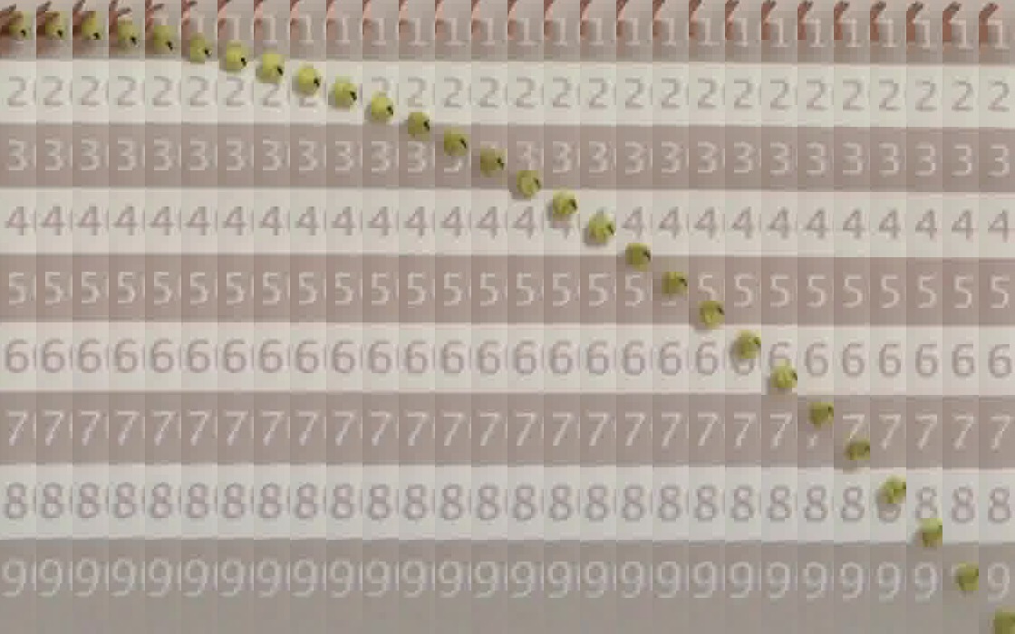
I made a web page with a timer and a distance scale, which was projected on the wall. The students used their cell phones to record a video of a falling ball. My version of the video is in YouTube. The key part of the video is summarized in the following picture.
With some tools that are explained on the original post, we got a table describing the distance travelled by the ball on each time. The distance column represents the vertical position in meters, and time is measured in seconds. There is some uncertainty on the distance, that I guess can be near 5cm. The time is more precise, as described in the experiment page. Our data looks like this:
freefall <- read.table("freefall_from_movie.txt",
                        header=TRUE)
plot(distance ~ time, data=freefall,
    main="Experimental data. Distance [m] v/s time [s]")
Since the ball distance follows a parabola, we would like to model it
with a formula like \[\mathit{distance}=\beta_2\cdot\mathit{time}^2+\beta_1\cdot\mathit{time}+\beta_0\]
Interestingly, we can fit this quadratic formula with a linear
modelNew concept: Quadratic linear
models.
. We need to add a new column, called
time_sq, with the time squared. Then we fit a linear
model.
freefall <- transform(freefall, time_sq=time^2)
model_fall <- lm(distance ~ time + time_sq, data=freefall)plot(distance ~ time, data=freefall,
main="Data and fitted quadratic model")
pred <- predict(model_fall)
lines(pred ~ time, data=freefall, col="red", lwd=2)
The fitted parameters of this model can be seen with the following commands
summary(model_fall)Call:
lm(formula = distance ~ time + time_sq, data = freefall)
Residuals:
Min 1Q Median 3Q Max
-0.02641 -0.00795 0.00133 0.00809 0.01970
Coefficients:
Estimate Std. Error t value Pr(>|t|)
(Intercept) 0.19495 0.00278 70.01 < 2e-16 ***
time 0.11290 0.02287 4.94 2.3e-06 ***
time_sq -5.03312 0.03934 -127.94 < 2e-16 ***
---
Signif. codes: 0 '***' 0.001 '**' 0.01 '*' 0.05 '.' 0.1 ' ' 1
Residual standard error: 0.011 on 133 degrees of freedom
Multiple R-squared: 0.999, Adjusted R-squared: 0.999
F-statistic: 1.2e+05 on 2 and 133 DF, p-value: <2e-16confint(model_fall) 2.5 % 97.5 %
(Intercept) 0.1894 0.200
time 0.0677 0.158
time_sq -5.1109 -4.955Your challenge is:
- Replicate this linear model from the same data
- You can use R, Excel or any tool of your preference.
- What is the meaning of each coefficient?
- What are the units of each coefficient?
- Calculate a 95% confidence interval for the acceleration of gravity.
- Does this interval match your background information?