1.1 Is this nucleotide G or C?

Please write a function called is_G_or_C that determines if a nucleotide is either “G” or “C”. The function takes a character vector (called dna) and returns a logic vector called ans. If dna[i] is “G”, “g”, “C” or “c”, then ans[i] is TRUE, otherwise it is FALSE.

is_G_or_C <- function(dna) {
    # write here
}

Test your function with the following code:

is_G_or_C(c("a","c","t","g"))

[1] FALSE  TRUE FALSE  TRUE

is_G_or_C(c("A","C","T","G"))

[1] FALSE  TRUE FALSE  TRUE

mean(is_G_or_C(c("A","C","T","G")))

[1] 0.5

As you can see, the GC content can be seen as the mean of the event is_G_or_C(). It is natural to think that we can also calculate the variance and the standard deviation. How can we do that?

1.2 Simulating some genes

We will use this function over simulated data. We need 100 genes of different lengths. Please create a vector, called sim_gene_length, with 100 elements taken randomly (with replacement) from the values 100, 103, 106, …, 1201. Then create a list, called sim_genes, with “random DNA sequences”Notice that sim_gene_length is a vector, since all elements are numbers. On the other side sim_genes has to be a list, since every element is itself a vector, and each one can have different length. We cannot handle this kind of data in a vector, it has to be a list.

. Each element sim_genes[[i]] must be a random character vector with length sim_gene_length[i]. Only the letters “A”,“C”,“G”, and “T” are valid, and all have the same probability.

After you have created sim_genes, calculate the mean of is_G_or_C() for each gene and store them in the vector sim_mean_GC. You also need to calculate the variance of is_G_or_C() for each gene and store the result in sim_var_GC.

Finally, calculate the standard error of the mean by taking the square root of sim_var_GC divided by sim_gene_length, and store it in sim_std_err_mean.

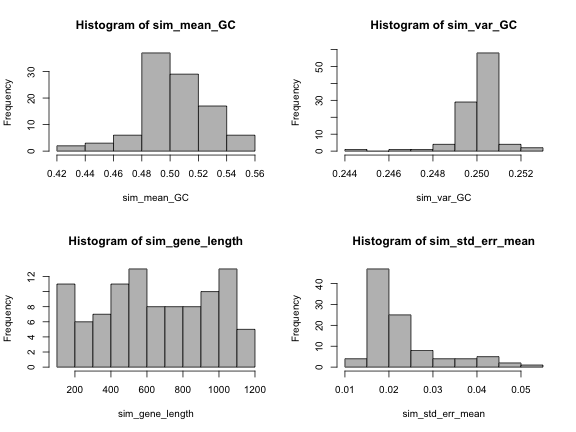
# write here

Test your results with this code:

par(mfrow=c(2,2))
hist(sim_mean_GC, col="grey")
hist(sim_var_GC, col="grey")
hist(sim_gene_length, col="grey")
hist(sim_std_err_mean, col="grey")

1.3 Genes versus genome

Since all genes are taking from a random population, and all nucleotides have the same probability, then in this case we know that the genome GC contentdo you agree?

is 0.5.

But in many cases we do not have the full genome, just some genes. We want use the information of each gene to build a confidence interval for the genome GC content.

Fortunately we know that, if the genes are random DNA sequences, the GC content of the genes is not too different from the GC content of the genomeWe know this because GC content is an average so they obey the Law of Large Numbers.

. Moreover, we know that the GC content of the genes is a random variable following the Normal distributionThis is true because of the Central Limit Theorem.

.

Unfortunately, we do not know the standard deviation of the population (we are using each gene as a sample). Instead, we can approximate it with the standard error of each geneStandard error of the sample is the standard deviation of the sample divided by the square root of the sample size \[\sqrt{\frac{\text{var}(x)}{\text{length}(x)}}\]

, but we will have to use the Student’s t distribution.

We start by choosing the confidence level \(1-\alpha=95\%\), therefore alpha is 0.05. You must use the function qt() to find the number of standard errors k that will give you the confidence interval. Remember that the number of degrees of freedom is sim_gene_length-1.

Then you must calculate the vectors sim_lower, with the lower limits of each confidence interval, and sim_upper, with the upper limits.

alpha <- 0.05
# write here

Now you can count how many of the confidence intervals really contained the real value. In other words, you can see how good was the prediction.

mean(sim_lower <= 0.5 & 0.5 <= sim_upper)

[1] 0.96

You can see your results with this code:

gene_order <- 1:length(sim_genes)
plot(gene_order, sim_mean_GC, pch=16, ylim=c(0.3, 0.7))
arrows(gene_order, sim_upper, gene_order, sim_lower,
       angle=90, code=3, length = 0.02)
abline(h=0.5, col="red")

The previous plot is hard to see, because there is a lot of variability. It can be a little easier if we use the function order() to sort the values, as in the following code:

sorted <- order(sim_mean_GC)
plot(gene_order, sim_mean_GC[sorted], pch=16, ylim=c(0.3, 0.7))
arrows(gene_order, sim_upper[sorted], gene_order, sim_lower[sorted],
       angle=90, code=3, length = 0.02)
abline(h=0.5, col="red")

2.1 Read the genes from a file

Please download the file c_rudii.fna.txt and save it in your computer. It has to be stored in your computer to be fast and efficient.

Using the library seqinr, please write the code to

• read the FASTA file and load all genes in a list called genes,
• calculate the mean of is_G_or_C() for each gene, and store each value in a vector called mean_is_G_or_C. The length of this vector must be the number of genes
• calculate the variance of is_G_or_C() for each gene, and store each value in a vector called var_is_G_or_C.
• calculate the length of each gene, and store each value in a vector called gene_length.
• calculate the standard error of the mean for each gene. That is, the square root of the variance divided by the gene length.

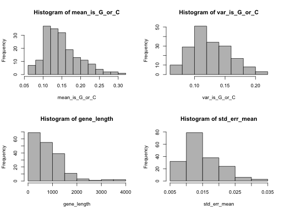
# write here

Test your results with this code:

length(genes)

[1] 182

par(mfrow=c(2,2))
hist(mean_is_G_or_C, col="grey")
hist(var_is_G_or_C, col="grey")
hist(gene_length, col="grey")
hist(std_err_mean, col="grey")

2.2 Using genes to estimate genome GC content

We want use the information of the real genes to build a confidence interval for the genome GC content.

Since the values have much more variability than in the simulation, we choose a confidence level of \(1-\alpha=99.9\%\), therefore alpha is 0.001. You must use the function qt() to find the number of standard errors k that will give you the confidence interval. Remember that the number of degrees of freedom is gene_length-1.

Then you must calculate the vectors lower, with the lower limits of each confidence interval, and upper, with the upper limits.

alpha <- 0.001
# write here

Test your results with this code:

gene_order <- 1:length(genes)
plot(gene_order, mean_is_G_or_C, pch=16, ylim=c(0, 0.4))
arrows(gene_order, upper, gene_order, lower,
       angle=90, code=3, length = 0.02)

The previous plot is hard to see, because there is a lot of variability. It can be a little easier if we use the function order() to sort the values, as in the following code:

sorted <- order(mean_is_G_or_C)
plot(gene_order, mean_is_G_or_C[sorted], pch=16, ylim=c(0, 0.4))
arrows(gene_order, upper[sorted], gene_order, lower[sorted],
       angle=90, code=3, length = 0.02)