Original paper by Réka Albert, The Plant Cell 19: 3327-3338 (2007)
The Main Goal of Systems Biology
A systems-level description of:
- The identity of the components constituting the biological system
- The dynamic behavior of these components
- The interactions among these components
Hypothetical Network Illustrating Network Analysis and Dynamic Modeling Terminology
Three concepts:
- Node
- Edges
- Node State
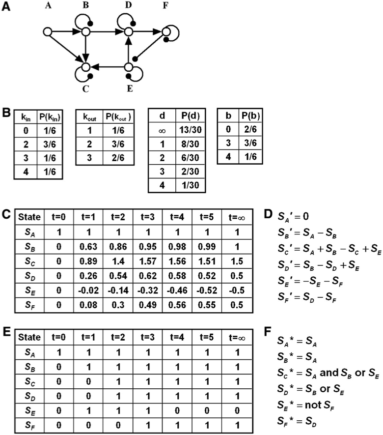
The interaction graph formed by nodes A to F consists of directed edges signifying positive regulation (denoted by terminal arrows), such as AB and ED, directed edges signifying negative regulation (denoted by terminal filled circles), such as FE and auto-inhibitory (decay) edges (denoted by terminal filled circles) at nodes B to F. The graph contains one feed-forward loop (ABC; both A and B feed into C) and one negative feedback loop, EDF, which also forms the graph’s strongly connected subgraph. The in-cluster of this subgraph contains the nodes A and B, while its out-cluster is the node C.
The node in-degrees (\(k_{in}\)) that quantify the number of edges that end in a given node range between 0 (for node A) and 4 (for node C). The node out-degrees (\(k_{out}\)), quantifying the number of edges that start at a given node, range between 1 (for C) and 3 (for B and E). The graph distance (\(d\)) between two nodes is defined as the number of edges in the shortest path between them. For example, the distance between nodes E and D is one, the distance between nodes D and E is two (along the DFE path), and the distance between nodes C and A is infinite because no path starting from C and ending in A exists. The betweenness centrality (\(b\)) of a node quantifies the number of shortest paths in which the node is an intermediary (not beginning or end) node. For example, the betweenness centrality of node A is zero because it is not contained in any shortest paths that do not start or end in A, and the betweenness centrality of node B is three because it is an intermediary in the ABD, ABDF, and ABDFE shortest paths. The in-(out-)degree distribution, [\(P(k_{in})\) and \(P(k_{out})\)] quantifies the fraction of nodes with in-degree kin (out-degree kout). For example, one node (C) has an out-degree of one; two nodes (E and F) have an out-degree of two and three nodes (A, B, and D) have an out-degree of three; the corresponding fractions are obtained by dividing by the total number of nodes (six). The distance distribution \(P(d)\) denotes the fraction of node pairs having the distance d. The betweenness centrality distribution \(P(b)\) quantifies the fraction of nodes with betweenness centrality b.
Hypothetical time courses for the state of each node in the network (denoted by \(S_A\) to \(S_E\)). The node states in this example can take any real value and vary continuously in time. The initial state (at \(t = 0\)) has state 1 for node A and 0 for every other node. Each node state approaches a steady state (a state that does not change in time), indicated in the last column (at \(t = \infty\)) of the time course. Network inference methods presented in section 2 use expression knowledge (such as the logarithm of relative expression with respect to a control state) such as this state time course to infer regulatory connections between nodes (i.e., the interaction network shown in [A]). State time courses like this also arise as outputs of continuous models.
The transfer functions of a hypothetical continuous deterministic model based on the interaction network (A) that leads to the time course under (C). Each transfer function indicates the time derivative (change in time) of the state of a node (denoted by a superscript ′ on the node state) as a function of the states of the nodes that are sources of edges that end in the node, including the node itself if it has an auto-regulatory edge. The transfer functions in this hypothetical example are linear combinations of node states, with a positive sign for activating edges and negative sign for inhibitory edges, and all coefficients (parameters) are equal to unity. In general, transfer functions are nonlinear and have parameters spanning a wide range.
Hypothetical discrete time courses for each node in the network, where the node states can only take one of two values: 0 (off) and 1 (on). Discrete states such as this are obtained using a suitable threshold and classifying expression values as below threshold (0) and above threshold (1). The initial state (at \(t = 0\)) has state 1 for node A and state 0 for all other nodes. As in (C), each node reaches a steady state, indicated in the last column (at \(t = \infty\)) of the time course. Binary time courses such as this form the basis of Boolean network inference methods presented in section 2. State time courses like this also arise as outputs of Boolean models.
The transfer functions of a hypothetical Boolean model based on the interaction network (A) that leads to the time course in (E). Each transfer function indicates the state of the node at the next time instance (\(t + 1\)), denoted by a superscript asterisk on the node state, as a logical (Boolean) combination of the current (time \(t\)) states of the nodes that are sources of edges that end in the node. In this case, the auto-inhibitory edges are not incorporated explicitly, assuming that positive regulation, when active, can overcome auto-inhibition. Decay (switching off) after the positive regulators turn off is taken into account implicitly by not including the current state of the regulated node in its transfer function. It is assumed that the state of the node A does not change in time. The inhibitory edge FE is taken into account as a “not SF” clause in the transfer function of node E. More than one activating edge incident on the same node in general can be combined by either an “or” or “and” relationship, depending on whether they are closer to being independent (in case of “or”) or conditionally dependent or synergistic (in case of “and”). In this example, the edges AC and BC are assumed to be synergistic and independent of EC, and the edges BD and ED are assumed to be independent of each other.
Focus
- Graph inference
- inferring interactions or functional relationships among a system’s elements and constructing the interaction graph underlying the system
- Graph analysis
- using the graph theory to analyze a known interaction graph and extracting new biological insights and predictions from the results
- Dynamic network modeling
- describing how known interactions among defined elements determine over time and in different conditions
These three topics have the same objective:
- to understand
- to predict
- and if possible to control
the dynamic behavior of biological interacting systems.
Inference of Interaction Networks from Expression Information
The most prevalent use of graph inference is using gene/protein expression information to predict network structure.
Genes with statistically similar expression profiles in time or across several experimental conditions can be grouped using clustering algorithms.
Clustering tool: Arabidopsis co-expression tool
The most highly co-regulated genes with WAT1 as identified with the Arabidopsis Co-expression Data Mining Tools from the University of Leeds (http://www.Arabidopsis.leeds.ac.uk/act/coexpanalyser.php). Nodes represent genes; edge width indicates whether two given genes are co-expressed above a certain mutual rank threshold. Nodes are color coded to reflect the level of induction by auxin of the corresponding genes according to the Genevestigator (https://www.genevestigator.com) and the Bio-Array Resource (http://www.bar.utoronto.ca) websites.
Graph-based inference
- Data analysis methods
- aim to highlight the global patterns in the expression of a large number of genes/proteins by condensing the multivariate data into just 3 or 3 composite variables.
- Principal component analysis
- The partial least-squares
- Bayesian methods
- aim to find a directed, acyclic graph describing the casual dependency relationships among components of a system and a set of local joint probability distributions that statistically convey these relationships.
- Model-based methods
- regulatory network inference from time-course expression data seek to relate the rate of change in the expression level of a given gene with the levels of other genes.
- Constraint-based deterministic methods
-
Performs metabolic pathway reconstruction from known reaction stoichiometric information.
- Flux balance analysis
- S-systems
Graph-based inference algorithms integrate indirect casual relationships and direct interactions to find the most parsimonious network consistent with all available experimental observations.
Network Analysis
- Metabolic networks
- have been represented in various degrees of detail, two of the simplest being the substrate graph, whose nodes are reactants and edges means co-occurance in the same chemical reaction and the reaction graph, whose nodes are reactions and edges means sharing at least one metabolite.
- Signal transduction networks
- involve both protein interactions and biochemical reactions and their edges are mostly directed, indicating the direction of signal propagation.
- Composite networks
- superimpose protein-protein and protein-DNA interactions, protein-protein interactions, genetic interactions, transcriptional regulation, sequence homology and expression correlation.
- Large-scale interaction networks
- The development of high-throughput interaction assays has led to the generation of large-scale interaction networks for a considerable number of organism.
The most often-used network measures describe the connectivity (reachability) among notes, the importance (centrality) of individual nodes, and the homogeneity or heterogeneity of the network in terms of a given node property.
Dynamic Modeling
Dynamic network models have as input:
- the interaction network
- the transfer functions describing how the state of each node depends on the its regulators
- the initial state of each node in the system
Dynamic modeling framework classification
- Continuous versus discrete
- Deterministic versus stochastic
Properties of a good model
- A low level of uncertainty in the interactions, equations, and parameters used
- Easy to run or construct
- Providing a high level of understanding or insight.
- Simplicity and elegance
- Highly accurate predictions
- Being general
- Robustness
Questions
- How much of graph based inference methods I should know?
- What knowledge level am I expected to in this course?
- Figure 1 and Figure 2 should be discussed in detail. There are parts that I could not understand.
- Should I better learn how to draw a graph? Going through graph theory?